A neural network is a model built from many neurons. The outputs of some neurons become the inputs of others, and the whole network is still one formula with parameters inside it. A neuron is the smallest piece, and a network is a model made by joining many of those pieces together. Every weight and every bias of every neuron is one parameter of the model. This page opens one neuron and works all of its arithmetic out with real numbers, so that nothing in the rest of the chapter stays a word you have to accept without checking it. The pages after it join neurons into networks.
You have met a neuron already without the name. The straight line fitted in what a model is is a neuron with one input and no rule at the end: its slope is a weight, and its offset is a bias. A neuron differs from that line in two ways. It can take several inputs, each with its own weight. And it passes its total through a simple rule before handing it on.
The neuron here reads the three readings of the first moment of the grasp example, in which the gripper is ready to close on a cup. When you reach the end of this page you will know which four numbers one neuron owns, what each of those numbers changes, and at which reading the neuron stops answering. The page ends on a limit that no choice of those four numbers can pass, because the line that divides the neuron's yes from its no is always straight. Activation functions is the page that passes that limit, so this page is what you need before that one.
Contents#
- What one neuron is made of
- The weighted sum, line by line
- What changes when a weight or the bias changes
- Where to read next
- Using it in Python
1. What one neuron is made of#
Before you can watch a neuron work, you need to know what goes into it and which numbers belong to it, and this section lays both out. The numbers that go into a neuron are called its inputs. The single number that comes out of it is called its output. Between the inputs and the output there are only four numbers, and those four numbers belong to the neuron itself.
The picture below follows one set of three inputs through the whole neuron, from left to right, and shows every number on the way.
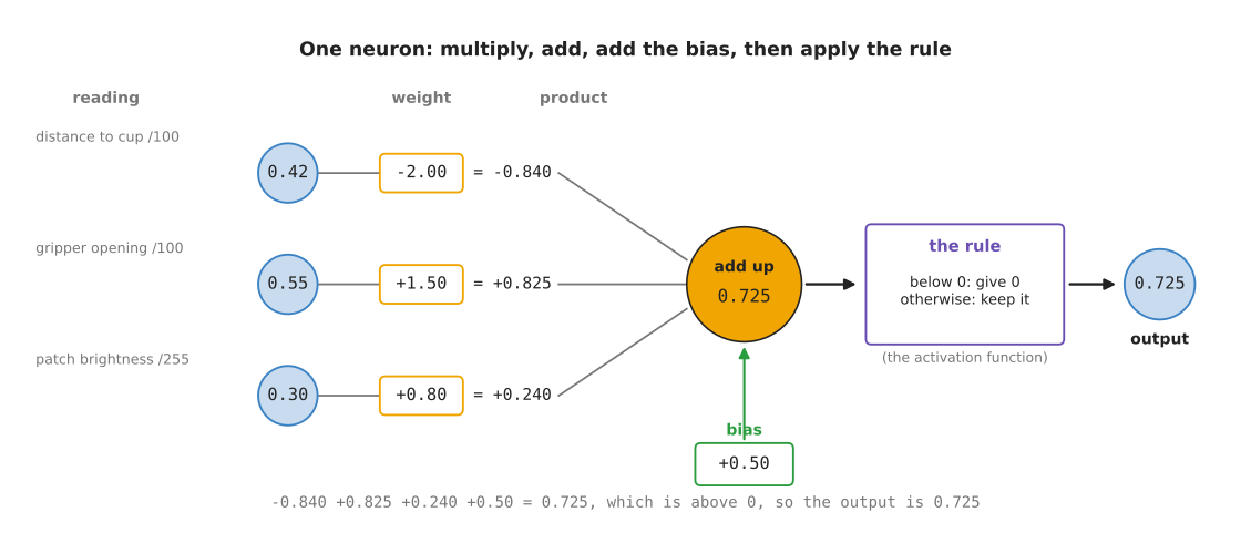
In that picture the three readings 0.42, 0.55 and 0.30 are multiplied by the three numbers -2.00, +1.50 and +0.80. The three results and one more number, +0.50, are added together, and they make 0.725. The rule at the end passes 0.725 through without changing it, because 0.725 is above 0.
The three inputs are the scaled readings of the arm: the distance to the cup, the gripper opening and the brightness straight ahead. The three readings says what each one measures and how it was scaled to sit between 0 and 1.
So the three numbers that reach the neuron are 0.42, 0.55 and 0.30. Now the four numbers that the neuron owns come in. Each input has one number of its own, which is called a weight. A weight says how much that input counts and in which direction. The neuron also has one further number, which is called its bias, and the bias is added to the total whatever the inputs are.
The weight on the distance is -2.00. The weight on the opening is +1.50. The weight on the brightness is +0.80. The bias is +0.50. These are the same four numbers that the first picture in this section showed in its boxes. That is four numbers for a neuron with three inputs.
A weight below 0 means that the neuron's answer gets smaller as that reading gets bigger. A weight above 0 means the opposite, so the answer gets bigger as that reading gets bigger. The weights here were picked so that this neuron answers one question, which is whether the arm is near a bright object with its gripper open. That combination is the moment when closing the gripper is likely to work. The distance has a minus weight because being far away counts against that moment. The other two readings have plus weights because they count in favour of it. In a real network nobody picks these four numbers by hand, because training picks them, and the chapter how training works explains that search.
The three readings here are of three different kinds: a distance, an opening and a brightness. Nothing requires that. A neuron only ever sees numbers, so its inputs can all be of one kind, such as sixteen pixel brightnesses. They can also be of different kinds, as they are here. What matters is that each reading is scaled first, so that no reading counts for more just because of its unit.
This page uses three readings so that you can follow the arithmetic by hand. A real robot might have 50 readings, and nobody decides which of them go to which neuron. In the usual layout, every neuron receives all 50 readings, and each neuron has 50 weights of its own. Training then sets those weights. When training leaves a neuron's weight on one reading close to 0, that neuron in effect ignores that reading. So the combination of readings that each neuron responds to is found by training, and no person chooses it. Layers, depth and width describes this layout, which is called a fully connected layer.
The inputs and the four numbers are now all on the table. The next section, the weighted sum, puts them together into the one number the neuron works with.
2. The weighted sum, line by line#
The section before gave the three inputs and the four numbers of the neuron, so the neuron can now do its first job. Everything else on this page changes one of these numbers and watches what happens to the result, so this calculation is the one to follow closely. That job is to work out the weighted sum, which means multiplying each input by its own weight, adding those results together, and then adding the bias. The whole calculation is short enough to write out completely.
distance     0.42  x  -2.00  =  -0.840      running total  -0.840
opening      0.55  x  +1.50  =  +0.825      running total  -0.015
brightness   0.30  x  +0.80  =  +0.240      running total  +0.225
bias                  +0.50  =  +0.500      running total  +0.725
The picture below is the same calculation as a table. Read it one row at a time, from left to right, and the last column keeps the total so far.
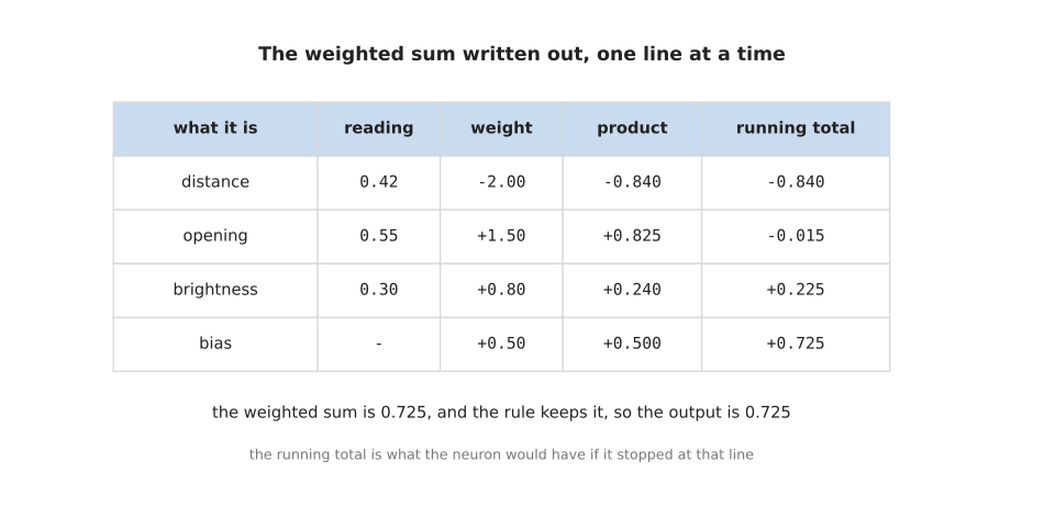
The three products are -0.840, +0.825 and +0.240. The bias adds +0.500 more. The running total after the last row is +0.725, and that number is the weighted sum.
The running total in the last column is worth following. After the distance alone the total is below 0. Only when the opening is added does the total rise back above 0. This is what a weighted sum does, because it lets several readings pull the answer in different directions, and the weights decide which reading pulls hardest.
The picture below draws each row of the table as one bar, so you can see which readings push the total up and which one pulls it down.
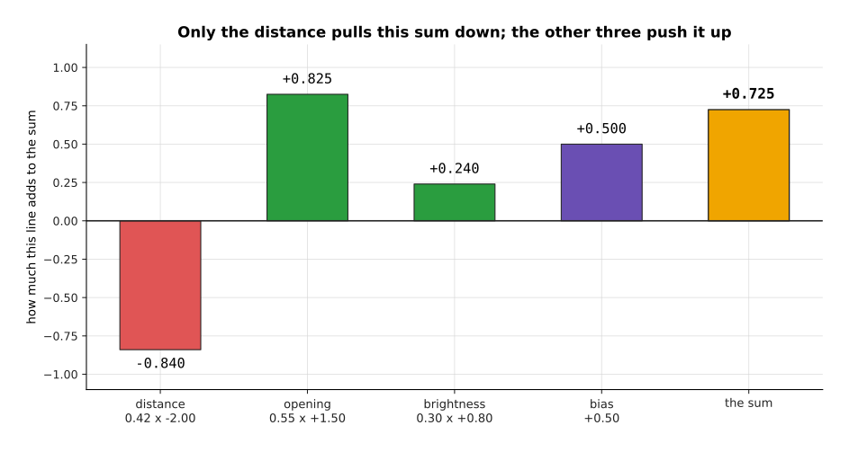
Only the distance pulls this sum down, because it is the only reading with a minus weight. The opening pushes the sum up the hardest, by +0.825.
The table and the bars describe one moment, with the cup standing still 42 millimetres from the palm. A robot does not stand still, so the useful question is how the sum changes as the readings change. The answer tells you where the neuron says yes and where it says no, and that dividing point is what the rest of this page is about. The next two pictures answer that question, first for one reading and then for two.
The next picture holds the opening at 0.55 and the brightness at 0.30, and it moves the scaled distance from 0 to 1, which is from 0 to 100 millimetres. Only one input changes, and that input is multiplied by one fixed weight, so the answer has to be a straight line. The line falls by exactly 2.00 for every 1.00 of scaled distance, because the weight on the distance is -2.00.
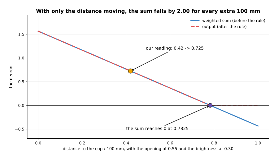
At a distance of 0 the sum is 1.565. At our reading of 0.42 it is 0.725. It crosses 0 at 0.7825, which is about 78 millimetres, and after that point the rule holds the output at 0.
That crossing point at 0.7825 is the distance at which this neuron stops answering. A neuron reads all of its readings at once, though, so one reading at a time does not show the whole decision. When two readings move together, the place where the sum crosses 0 is no longer a single point. It becomes a line across the picture, with yes on one side of it and no on the other.
The picture below sweeps the distance along the bottom and the gripper opening up the side. The colour gives the weighted sum at each pair of readings, and the black line marks every pair where the sum is exactly 0.
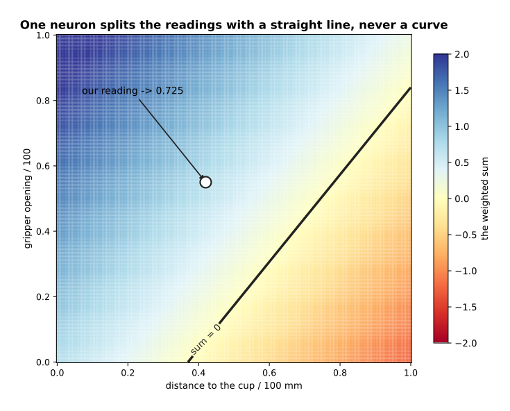
Over the whole square the sum runs from -1.260 to +2.240. The line where the sum is exactly 0 reaches an opening of 0.84 at a distance of 1, and it leaves the square through the bottom edge. Our own reading sits well inside the part where the sum is above 0.
The straightness of that line is the most important limit of a single neuron, and why multiplying and adding is not enough returns to it. Before that, the next section, what changes when a weight or the bias changes, moves that line by changing the neuron's four numbers, because those four numbers are the only thing training can change.
3. What changes when a weight or the bias changes#
The section before ended with a straight line that divides yes from no. This section asks what moves that line. The question matters because training, which the next chapter explains, does nothing except change weights and biases. So what these four numbers control is everything that training can do to one neuron.
This section changes one of the four numbers at a time and shows what the neuron does differently. There are three things to see. The sign of a weight decides what the neuron is for. The size of a weight decides how much the neuron cares about that reading. The bias decides where the neuron stops answering.
Start with the sign. Keep the same three readings, and change the weight on the distance from -2.00 to +2.00. The distance row then gives +0.840 instead of -0.840, and the sum rises from +0.725 to +2.405. With the minus weight the neuron answers whether the arm is close to the object. With the plus weight it answers whether the arm is far from it. The robot did not change, and only one weight did.
Now the size. The picture below draws the line where the sum is exactly 0, for three sizes of the weight on the distance. The other numbers stay as they were.
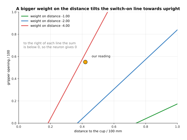
The bigger the weight, the closer to upright the line stands. An upright line means that the distance alone decides whether the neuron is on, and the opening hardly matters.
Last, the bias. It is added whatever the readings are, so it moves the line without tilting it. The picture below shows this with only the distance moving.
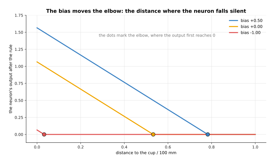
With the bias +0.50 the output reaches 0 at a distance of 0.7825, which is about 78 millimetres. With 0.00 it reaches 0 at 0.5325, about 53 millimetres. With -1.00 it reaches 0 at only 0.0325, about 3 millimetres. So a lower bias makes the neuron stop answering at a shorter distance.
Those four numbers are the only freedom this neuron has. Whatever you do to them, the dividing line stays straight. That is where this page stops. Why multiplying and adding is not enough shows why a straight line is a problem, and why the rule at the end of the neuron is the thing that solves it. Before that, the smallest network joins four neurons like this one into a network.
4. Where to read next#
- The smallest network is the next page. It puts this neuron in a layer with three others and works the same moment through the whole network.
- Activation functions takes the straight dividing line that this page ended on and shows the one small rule that lets a neuron bend it.
- Layers, depth and width joins many copies of this neuron into a layer, stacks those layers, and explains what each extra layer adds and what it costs.
- The shape of the numbers explains how these weights are stored and multiplied, and why the hardware is built the way it is.
- The score of being wrong starts the chapter that searches for the weights and biases this page chose by hand.
- Inside a neural network is the short version of the same ideas in the catalogue of models, and it carries on into the layer types used for pictures and sentences.
5. Using it in Python#
Everything on this page is one line of PyTorch, which is the library most of this book's models are built with. The code below builds the same neuron as what one neuron is made of, puts the same three readings through it, and checks the arithmetic of the weighted sum.
import torch
from torch import nn

neuron = nn.Linear(in_features=3, out_features=1)   # 3 weights + 1 bias
with torch.no_grad():                               # fix them by hand, as this page did
    neuron.weight.copy_(torch.tensor([[-2.0, 1.5, 0.8]]))
    neuron.bias.copy_(torch.tensor([0.5]))

readings = torch.tensor([[0.42, 0.55, 0.30]])       # the three scaled readings
total = neuron(readings)                            # the weighted sum
print(f"{total.item():.4f}")                        # 0.7250
print(sum(p.numel() for p in neuron.parameters()))  # 4
The class is called nn.Linear and not nn.Neuron, because it is written to hold
a whole layer of neurons at once. Asking for one output is how you get a single
neuron out of it. The library gives you the weights, the bias, the multiplying and
the adding, so you never write the arithmetic of
the weighted sum yourself.
Each number is printed to four decimal places on purpose. PyTorch works in a number format called float32, which keeps only about seven digits, so the full printout would end in digits that depend on the order in which the machine added things up. The page the shape of the numbers explains that format and the smaller ones that models are run in.
What you have to decide is none of the arithmetic and all of the shape. You choose how many inputs the layer takes and how many neurons it has, which layers, depth and width is about. You also choose which rule to apply after it, which activation functions weighs up. You do not choose the weights or the bias, because training chooses those.