One neuron worked a single neuron out by hand, and activation functions added the rule that lets it bend. Three readings from a robot arm were each multiplied by a weight, the results and a bias were added together to make 0.725, and the rule decided what came out. This page comes next because one neuron is still not a model. It gives one number, and it can only ever draw a straight line across its readings. This page puts many neurons side by side into a layer, stacks layers one after another, and answers the question that follows from doing so, which is what each extra layer gives you. What it costs you is arithmetic on the same example, and that is worked out on the page after this one, layers, depth and width, worked out.
Three words do most of the work on this page. A layer is a group of neurons that all read the same numbers. The width of a layer is how many neurons it has. The depth of a network is how many layers it has, one after another. Choosing the width and the depth is most of what a person actually decides when they build a network, so this page shows what each of the two choices gives you.
When you reach the end you will know what a layer is, what makes a layer fully connected, why a second layer is not the same thing as a wider first one, what depth and width each add, and what one small change makes a deep stack trainable at all.
Contents#
- A layer is many neurons reading the same numbers
- Fully connected, and what joining everything costs
- What a second layer gives you
- Depth and width, and what each one changes
- Residual connections
- Where to read next
- Using it in Python
1. A layer is many neurons reading the same numbers#
The layer comes first because every later idea on this page is built from it. The neuron on the page before this one answered one question about the grasp, and a robot needs more than one answer. So the first step is to put several neurons side by side and to give all of them the same three readings. That group of neurons is a layer. The only new idea in it is that each neuron keeps its own weights and its own bias, so the same three numbers going in come out as several different answers.
The picture below draws four neurons that all read the same three readings. Each line carries one reading to one neuron, and each box holds that neuron's own weights, its bias, its sum and its output.
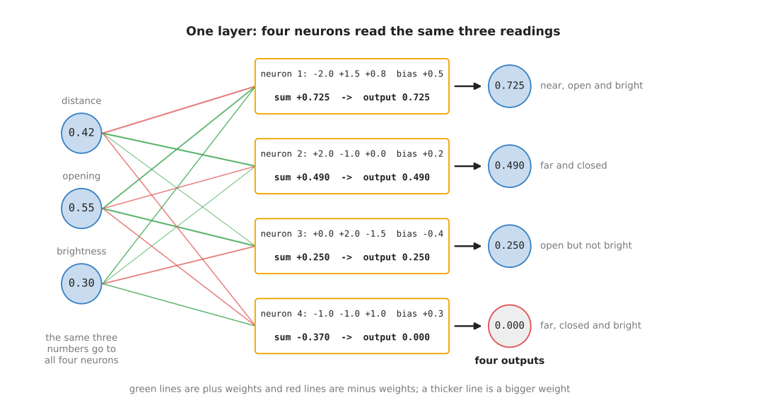
The same readings 0.42, 0.55 and 0.30 reach all four neurons. The four sets of weights are different, so the four sums are different as well: they are +0.725, +0.490, +0.250 and -0.370. The rule turns those sums into the outputs 0.725, 0.490, 0.250 and 0.000.
Nothing in that picture is new arithmetic, because it is the weighted sum of the page before done four times over. It is still worth writing out once, because seeing all twelve products at the same time is what makes a layer one thing rather than four.
The picture below is a table with one row for each neuron. Read each row from left to right: the three products, then the bias, then the sum of all four, then the output after the rule.
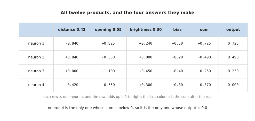
Neuron 2 has the products +0.840, -0.550 and +0.000 and the bias +0.20, and those four numbers make +0.490. Neuron 4 reaches -0.370, and it is the only neuron that the rule silences.
The twelve weights are usually drawn as a grid rather than as four separate lists, with one row for each neuron and one column for each input. They are drawn that way because that is how a computer stores them, and because that is how the next page describes them.
The picture below shows that grid, with the four biases in a column beside it.
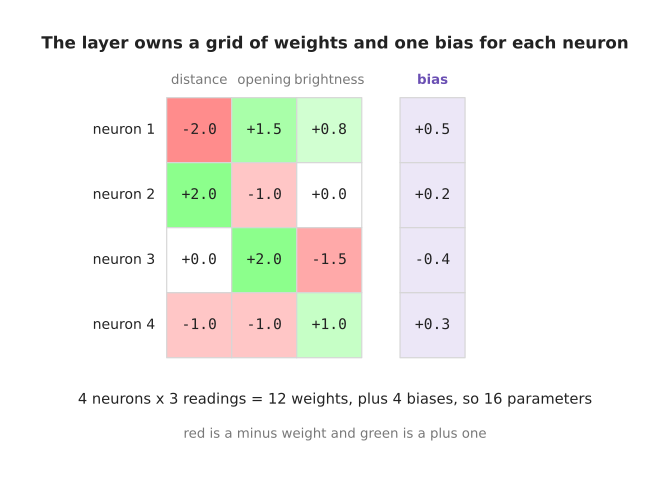
Four neurons reading three numbers need 4 times 3 weights, which is 12 weights. Each neuron also has one bias, which is 4 more numbers. So the whole layer owns 16 numbers, and those numbers are called its parameters.
The four numbers that come out of the layer are the layer's features, the word neural networks and neurons introduced for a number worked out from the readings that says something useful about them. The point of having four features is that each one describes the moment in a different way, so together they say more than any one of them could.
The picture below draws those four outputs as four bars, with the sum that produced each one written underneath it.
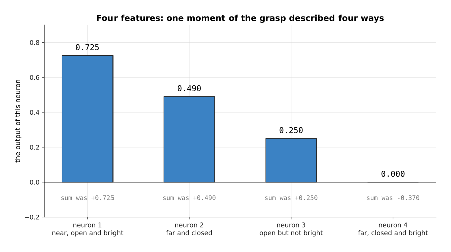
Three readings have become four features. The fourth feature is 0.000, because its sum of -0.370 was below 0. That neuron is saying nothing at all about this particular moment.
In this layer the weights were chosen by hand, so that each neuron has a description you can read. In a trained network nobody chooses them, so nobody can say in advance what each feature will mean.
This layer joined every reading to every neuron, so the next section asks what that arrangement is called and what it costs as the layer grows.
2. Fully connected, and what joining everything costs#
This section comes now because the layer of four neurons joined every reading to every neuron, and that arrangement has a name. It is called a fully connected layer, and it is also called a dense layer or a linear layer. It is the plainest layer there is, because it assumes nothing about what the inputs mean and it lets every neuron look at every one of them.
The picture below draws that layer again with the arithmetic left out, so that only the lines are left to count.
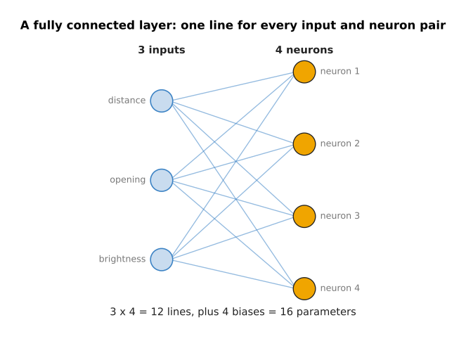
Three inputs into four neurons is 3 times 4 lines, which is 12 weights, plus 4 biases, which makes 16 parameters. Six inputs into eight neurons would be 48 weights plus 8 biases, which makes 56. So the count is the number of inputs multiplied by the number of neurons, plus one more for each neuron.
That multiplication is the whole cost of a fully connected layer. The layer of four neurons is small enough to draw, but the layers in real models take hundreds or thousands of numbers in, and then the count grows quickly.
The picture below holds the number of inputs at 1,024 and changes the number of neurons. On both axes an equal step means an equal multiplication rather than an equal addition, because the counts are too far apart for ordinary axes.
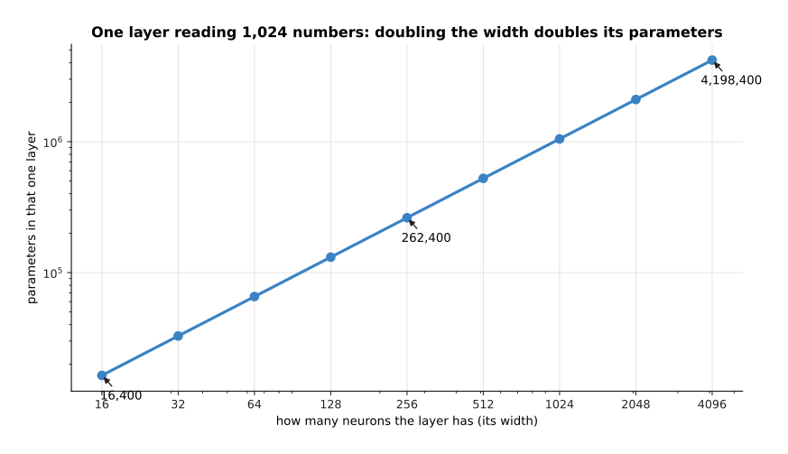
A layer that reads 1,024 numbers has 16,400 parameters when it has 16 neurons, 262,400 parameters when it has 256, and 4,198,400 parameters when it has 4,096. Doubling the number of neurons doubles the count.
Joining everything to everything is a poor choice when the inputs have a shape of their own. If the inputs are the pixels of a picture, then two pixels next to each other are related, and two pixels at opposite corners usually are not. A fully connected layer has no way of knowing that, so it has to learn it from the examples.
The picture below draws sixteen inputs joined to sixteen neurons in the fully connected way, with every pair joined.
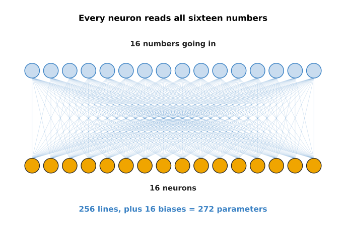
That wiring draws 256 lines, which is 256 weights, and 16 biases, so it has 272 parameters.
The picture below draws the same sixteen inputs and sixteen neurons again. This time each neuron reads only three numbers, which are the input at its own place and the two inputs beside it.
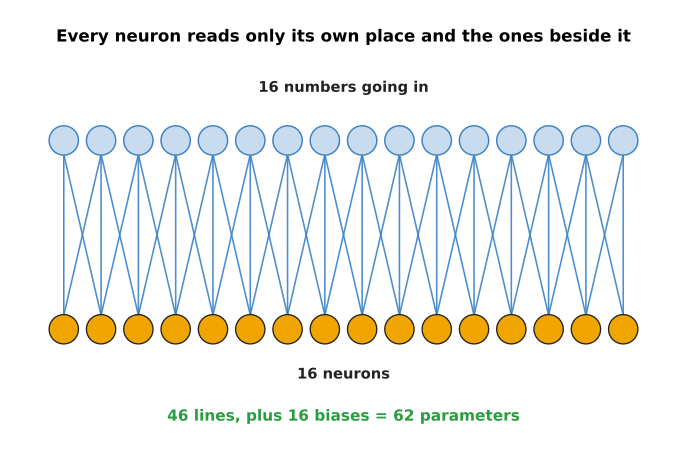
That wiring draws 46 lines rather than 48, because the neuron at each end of the row has only one neighbour instead of two. With the 16 biases it has 62 parameters in all, which is 4.4 times fewer than the 272 above.
That second arrangement, repeated with the same weights at every position, is called a convolution, and it is the subject of what a network can learn. All this page says about it is that a fully connected layer is the general case, and that the special layers are savings made by knowing something about the input.
This section counted what one layer costs, so the next section asks what a second layer could give you that is worth paying that cost again.
3. What a second layer gives you#
With the cost of one layer counted, the question now is why anybody would use more than one layer. The answer is that the second layer does not read the readings. It reads the features that the first layer made, and that is a different thing to read.
The picture below shows this directly. The four circles on the left are the four features from the first layer, and three new neurons read them.
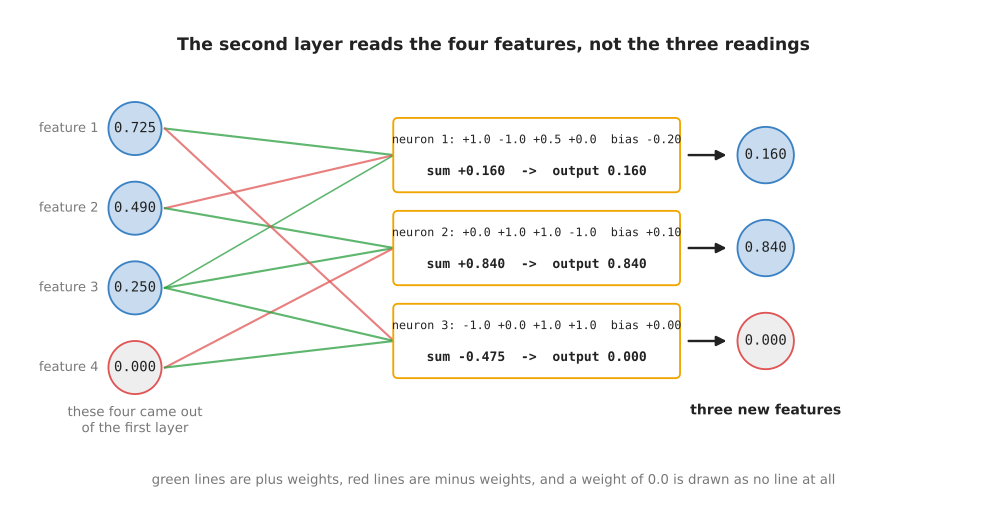
Those three second-layer neurons give the sums +0.160, +0.840 and -0.475, so after the rule their outputs are 0.160, 0.840 and 0.000. The camera readings of 0.42, 0.55 and 0.30 appear nowhere in that arithmetic, because the second layer never sees them.
Activation functions showed, in why multiplying and adding is not enough, that two layers with nothing between them collapse into one layer, so everything in this section assumes that the rule is applied after each layer.
To see what the second layer adds, it helps to count bends. A bend is a place where a line changes direction. Activation functions showed, in the rectified linear unit, that each neuron with the rule has one such place of its own.
The picture below sweeps the patch brightness from 0 to 1 and draws what one layer of two neurons gives.
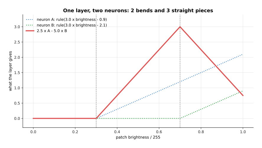
The two neurons have their bends at 0.300 and 0.700, so the line they make together has 2 bends and 3 straight pieces. No choice of the numbers that combine them can give it more.
Now add a second layer of two neurons that reads those two features instead of the brightness. The neurons in the second layer have bends of their own, but a bend in the second layer appears wherever the first layer's output crosses the second neuron's switching point. So the new bends land in places where neither first-layer neuron has a bend.
The picture below draws what each of the two second-layer neurons gives, against the brightness that neither of them reads.
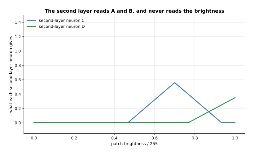
Neither of those two lines bends at 0.300, which is where the first layer bends.
The picture below adds the two second-layer neurons together and draws the answer of the whole two-layer network, with the one-layer answer behind it for comparison.
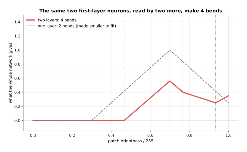
The same two first-layer neurons, read by two more neurons, give a line with 4 bends instead of 2. The bends sit at 0.467, 0.700, 0.767 and 0.933, and three of those four are at brightness values where the first layer had no bend at all.
That is the mechanical answer. The useful answer is what the layers end up meaning. When researchers look inside a trained network for pictures, they find the same pattern again and again. The neurons in the early layers answer questions about edges and patches of colour. The neurons in the middle layers answer questions about shapes made of those edges, such as corners and curves. The neurons in the late layers answer questions about whole parts of objects, such as a handle or a rim. Nobody tells the network to do this, because it comes out of training on its own.
The three stages below are built by hand, so that the arithmetic stays visible. They work on a simulated picture of a cup with a handle, 14 pixels by 14 pixels, in which 1 is bright and 0 is dark.
The picture below shows the cup on the left and the first stage's answer on the right. The first stage slides nine weights over the picture, one place at a time, and at each place it asks whether a dark column is followed by a bright one.
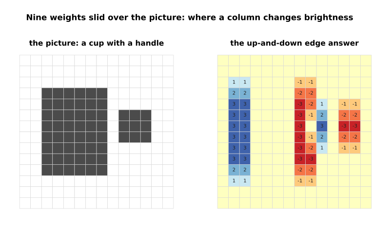
That filter gives +3 where a dark column is followed by a bright one, and -3 where a bright column is followed by a dark one. It is positive in columns 1, 2 and 9, and it is negative in columns 7, 8, 11 and 12.
The picture below shows the same cup again, with the same nine weights turned sideways so that they ask about rows instead of columns.
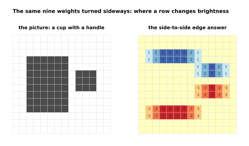
That filter answers along the top and the bottom of each shape, on rows 2, 3, 4, 5, 7, 8, 10 and 11.
Nothing in that first stage knows anything about cups, because each answer comes from nine numbers at one place. The second stage reads the first stage's two answers rather than the picture. It asks whether there is an up-and-down edge and a side-to-side edge in the same place, which is what a corner is.
The picture below shows the cup beside the second stage's answer, with the places where the answer rises above 2 outlined.
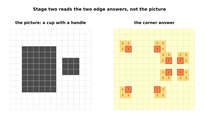
The corner answer rises above 2 at exactly 8 places, which are the four corners of the body and the four corners of the handle.
The third stage also reads the first stage rather than the picture. It asks whether there is a dark-to-bright edge with a bright-to-dark edge two columns further to the right, which is what a bright bar three columns wide looks like.
The picture below shows the cup beside the third stage's answer, with the places where it answers above 0 outlined.
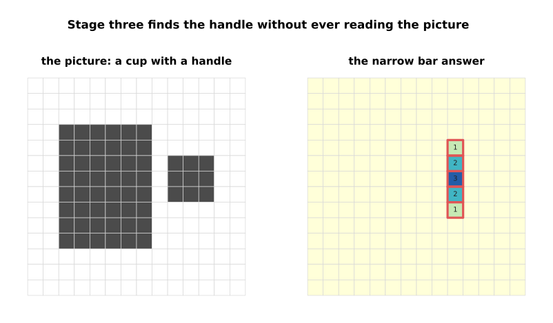
The narrow-bar answer is above 0 at 5 places, and all five are in the handle. It is 0 everywhere on the body, because the body is six columns wide and this question only accepts three.
So the third stage has found the handle, and it found the handle without ever looking at the picture, because it only looked at what the first stage said. That is what an extra layer gives you. It does not give you more lines across the readings. It gives you questions asked about the answers to earlier questions.
A second layer adds bends and new questions, so the next section asks how far that goes as you add more layers or more neurons in each one.
4. Depth and width, and what each one changes#
This section comes now because the second layer added something, and the next step is to measure how much more layers and wider layers each add. Answering it means measuring the two words in this page's title. The depth is how many layers a network has, and the width is how many neurons each layer has.
The picture below names both of them on one small stack, of the shape this page has been building.
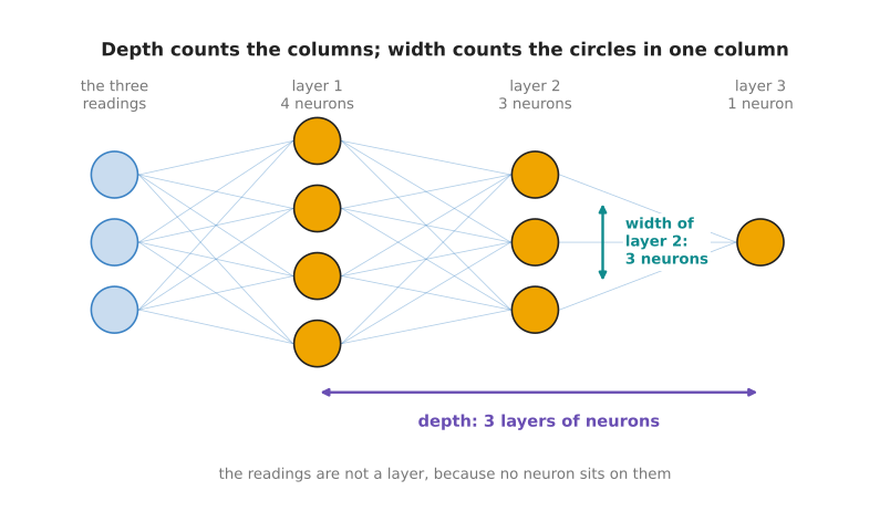
That stack has 3 layers of neurons, and their widths are 4, 3 and 1. The three readings are not a layer, because no neuron sits on them. A network that is called deep is simply one with many layers, and that is where the name deep learning comes from. There is no exact number at which deep starts, although vision models often have dozens of layers and the largest language models have around a hundred.
One way to measure what a network can do is to count the straight pieces its answer is made of, because what a second layer gives you showed that a network changes direction only where a neuron has a bend. In the pictures below a single reading is swept from -1 to +1. The weights are drawn at random from a fixed starting point, the pieces are counted by the script on a sweep of 6,001 points, and each number is the average over five networks of the same shape.
The picture below holds the width at 8 neurons and changes the depth.
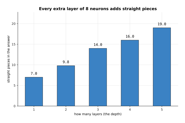
One layer gives 7.0 pieces on average, two layers give 9.8, three give 14.0, four give 16.0 and five give 19.0. So every extra layer adds more detail to the answer.
The picture below draws the answers that two of those networks actually make, so that you can see what a piece is.
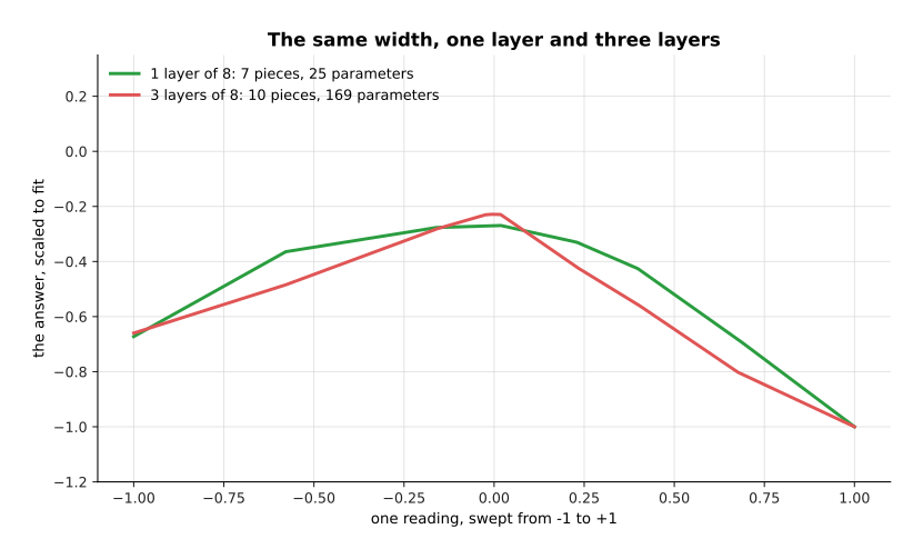
The one-layer network in that picture has 25 parameters and makes 7 pieces. The three-layer network has 169 parameters and makes 10 pieces. Both answers are drawn at the same height on purpose, because only their shape is being compared.
Width does the same job in a different way, because each neuron in a layer has one bend of its own. So adding neurons to a layer adds places where the answer can change direction.
The picture below changes the width instead of the depth, for networks of one layer and of two.
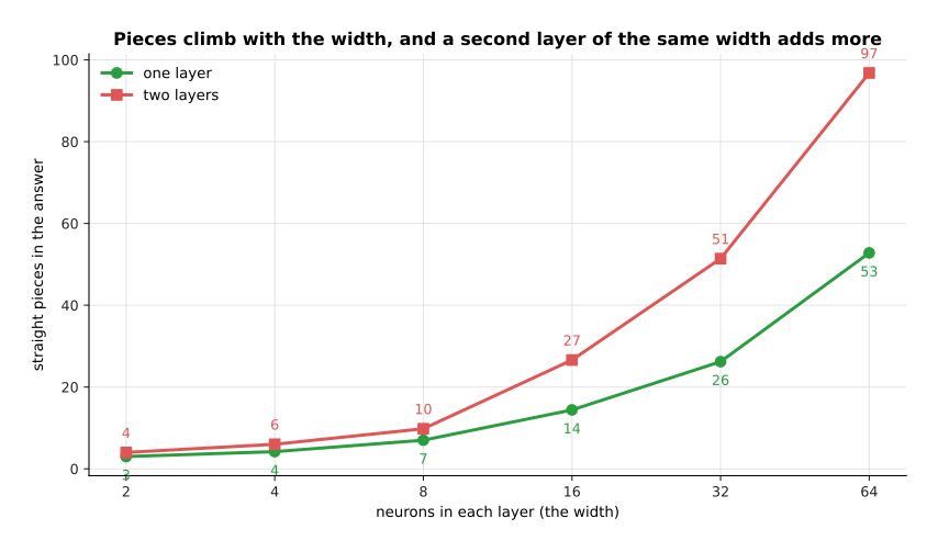
One layer of 8 neurons gives 7.0 pieces and one layer of 64 gives 52.8. Two layers of 8 give 9.8 and two layers of 64 give 96.8. So a greater width raises both lines, and the second layer raises them again.
The two measurements can be put together, and the answer to which of them is worth more is less exciting than it might be.
The picture below is a grid. Each row is one depth, each column is one width, and the number in a cell is the pieces that shape makes on average.
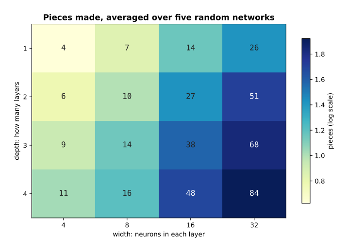
The picture below takes those same sixteen numbers and plots each of them against the total number of neurons in that network, which is the depth multiplied by the width.
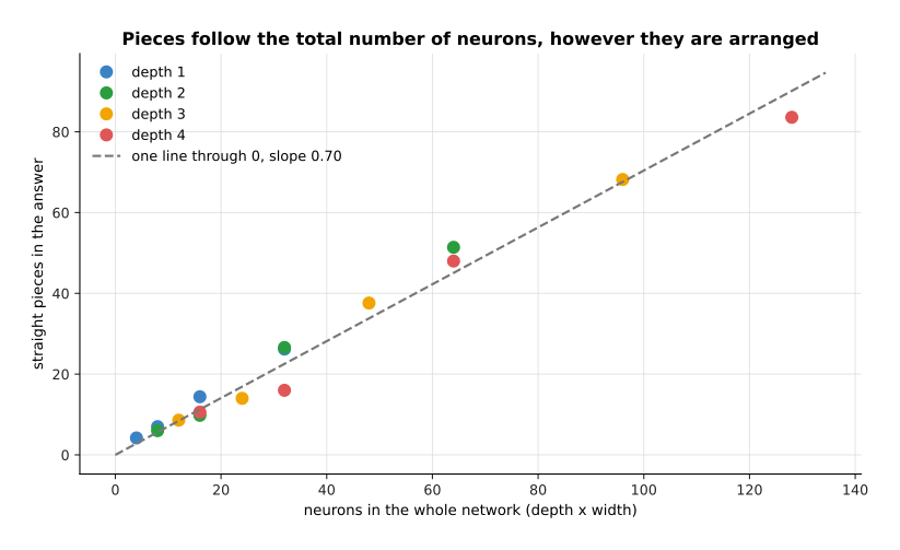
All sixteen shapes lie close to one straight line through zero with a slope of 0.70. That means that with weights picked at random it is the total number of neurons that decides the detail, and not how those neurons are arranged into layers.
That is worth saying plainly, because it is easy to be told that depth is powerful and then to believe that a deep network is better at everything. Two networks with about the same number of parameters can be arranged either way, and with random weights the flat one is not behind.
The picture below draws the answers made by one deep narrow network and one flat wide network.
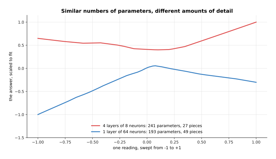
Four layers of 8 neurons have 241 parameters and make 27 pieces. One layer of 64 neurons has 193 parameters and makes 49 pieces. So on this measure the wide flat network is ahead, with fewer parameters.
What the deep network has instead is what the stages that found the handle showed, which is layers that ask questions about earlier answers. That advantage only appears once training has chosen the weights, and these weights were not trained. So the short answer is this. Width gives a layer more different features at the same stage. Depth gives later stages something built to ask about. Real models use plenty of both.
Both depth and width add detail, so the question that follows is what each one costs, because cost is what decides between them. That is arithmetic rather than a new idea, so it is worked out on the next page, in what depth and width cost. The short version, which the section below needs, is that a wider layer costs four times as much for each doubling and a deeper stack only twice as much, so adding layers is the cheaper way to buy detail.
5. Residual connections#
This section comes now because adding layers is the cheaper choice, as the sentence above said, and that choice only works if a deep stack can be trained. When deep networks were first built, making a plain stack deeper than a few dozen layers made it worse rather than better. It was worse even on the examples it had been trained on, which is not the usual failure of a model that has too many parameters. The fix is one of the smallest changes in this book. Instead of passing each layer's output on, you add that output to the layer's input and pass the total on. That addition is a residual connection, and a layer wrapped in one is usually called a block.
The picture below works one such block out on four numbers. The four numbers enter on the left, the block works out four numbers of its own, the line along the top carries the original four to the end, and the two sets are added together.
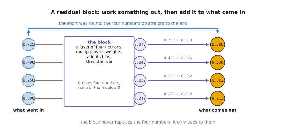
The four features from the first layer were 0.725, 0.490, 0.250 and 0.000. They go into a small block, which answers 0.073, 0.046, 0.052 and 0.212. The output is the two sets added together, which is 0.798, 0.536, 0.302 and 0.212.
The thing to notice is that the output can never be further from the input than the block's own answer, because the block adds to what it was given instead of replacing it. The effect builds up over a stack. The easiest way to see it is to push one set of 64 numbers through 30 layers twice, once through a plain stack and once through a residual stack, using the same randomly drawn weights both times.
The picture below does that and draws the typical size of the numbers after every layer. The side axis grows by a factor of ten at each step, because the two lines end up very far apart.
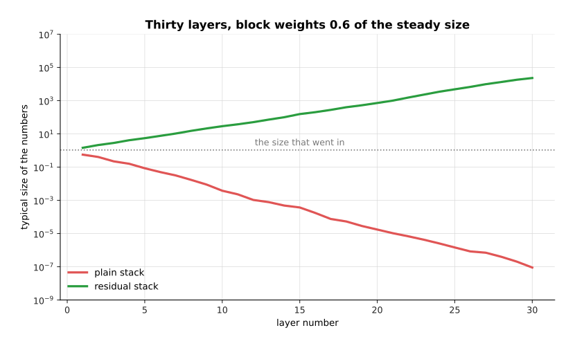
In that picture the block weights are 0.6 of the size that would hold the numbers steady. Numbers with a typical size of 1.071 go in. After 30 plain layers they are 0.0000000896, and after 30 residual layers they are 23,100.
Those numbers are worth reading carefully, and they change when the weights change, so the picture below gives them as a table at five depths and at two weight sizes. Read one row at a time: the row says which layer the numbers were read after, and the four columns give the plain stack and the residual stack at each of the two weight sizes.
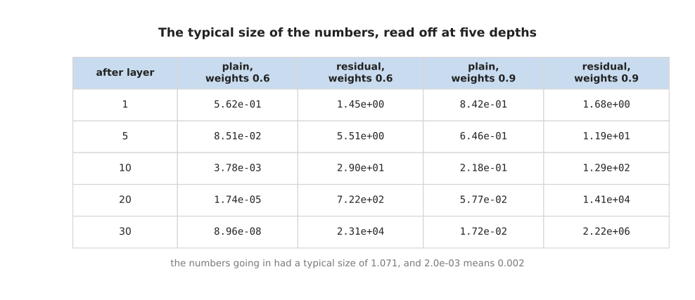
The plain stack with weights 0.6 falls from 0.562 after one layer to 0.0000000896 after thirty, so by the end the numbers are millions of times smaller than what went in. The residual stack with the same weights rises from 1.45 to 23,100. With the larger weights of 0.9 the plain stack ends at 0.0172 and the residual stack ends at 2,220,000.
Neither of those two results is good on its own. The plain stack loses everything that went in if the weights are a little too small, and the residual stack grows instead. That is why every real network puts a step inside each block that rescales the numbers. That step is called normalisation, and normalisation and stability explains it. With that step in place, a residual stack holds its numbers steady for hundreds of layers.
What the addition really gives you appears in the case where the block has almost nothing to say, which is where a plain layer does the most damage. In the two pictures below the weights are a hundred times smaller than usual, and the first twelve of the 64 numbers are drawn before and after.
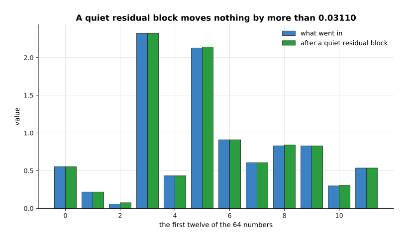
With those tiny weights the residual block moves no number by more than 0.031, so what came in is still there at the end.
The picture below uses the same twelve numbers and the same tiny weights, but without the addition.
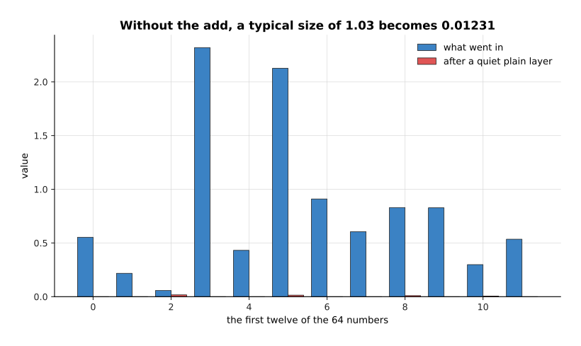
The same weights in a plain layer shrink the typical size from 1.033 to 0.012, which leaves almost nothing.
So a residual block can do nothing, and a plain layer cannot. Adding a block to a network that already works can leave it working, which means that a deeper network starts out at least as good as a shallower one and can only improve from there. That is what made stacks of fifty, a hundred and more layers trainable. Almost every model in this book is built from blocks of this shape, including the transformer block that the chapter the transformer explains part by part.
This page has now built layers, stacks and blocks, so the pages below take each of those ideas further.
6. Where to read next#
Each page below picks up one idea from this page and explains it in more depth.
- Layers, depth and width, worked out is the next page. It counts the parameters and the arithmetic of the layers on this page, which is how the choice between depth and width is actually made.
- The shape of the numbers explains how the weight grid is stored, what a matrix multiply is, and why the hardware that runs models is built around it.
- What a network can learn explains why stacking these layers can follow any shape at all, and it introduces the convolution that fully connected, and what joining everything costs compared a fully connected layer against.
- A transformer block is the residual block as it is actually built today, with attention inside it.
- Normalisation and stability explains the rescaling step that keeps the numbers in the residual stack from growing.
- Backpropagation explains the training problem that residual connections were invented to solve.
- Inside a neural network gives the same layer ideas in short, next to the catalogue of models that use them.
7. Using it in Python#
A layer, a stack of layers and a residual block are each a few lines of PyTorch. The code below builds the layer of four neurons with the same weights, counts its parameters, counts a bigger stack from what depth and width cost, and wraps a block in the addition of residual connections.
import torch
from torch import nn

layer = nn.Linear(3, 4)                     # the first layer: four neurons, three inputs each
with torch.no_grad():                       # the same weights this page used
    layer.weight.copy_(torch.tensor([[-2.0, 1.5, 0.8], [2.0, -1.0, 0.0],
                                     [0.0, 2.0, -1.5], [-1.0, -1.0, 1.0]]))
    layer.bias.copy_(torch.tensor([0.5, 0.2, -0.4, 0.3]))

readings = torch.tensor([[0.42, 0.55, 0.30]])
sums = layer(readings)[0]                   # the first layer: the four weighted sums
print([f"{v:.3f}" for v in sums])           # ['0.725', '0.490', '0.250', '-0.370']
print([f"{v:.3f}" for v in torch.relu(sums)])   # ['0.725', '0.490', '0.250', '0.000']
print(sum(p.numel() for p in layer.parameters()))   # 16

layers = []                                 # the cost: a stack of 8 layers of 1024
for _ in range(8):
    layers += [nn.Linear(1024, 1024), nn.ReLU()]
stack = nn.Sequential(*layers)
print(sum(p.numel() for p in stack.parameters()))   # 8396800

class Block(nn.Module):                     # the residual block: one block
    def __init__(self, width):
        super().__init__()
        self.inner = nn.Sequential(nn.Linear(width, width), nn.ReLU())

    def forward(self, x):
        return x + self.inner(x)            # the addition is the whole idea
The library gives you the weight grid, the bias, the multiplying and the adding,
and nn.Sequential gives you the stacking. So a network of 8 layers is one line,
and its parameter count comes back as 8,396,800, which is the number what depth
and width cost counted. The residual block needs a class of its own only because
nn.Sequential passes each output straight on and has nowhere to keep the input.
What you decide is the shape. You choose the width of each layer and how many layers there are, which depth and width, and what each one changes and what depth and width cost weighed up. You choose whether the layers are fully connected or one of the special kinds that the next pages describe. You also choose whether to wrap each layer in a residual addition, and for anything deeper than a few layers the answer is yes.
What you do not decide is any of the numbers inside. The weights above were copied in by hand so that the printout matches this page. In every real model they start as small random values and are changed by training, which the chapter how training works explains from the beginning.