The page before this one, the shape of the numbers, showed three things. It showed that a fully connected layer is one matrix multiply. It showed that a batch of examples goes through that layer in a single operation. It showed that the memory a model needs is its parameter count multiplied by the bytes each parameter takes. All three of those facts are about cost. This page comes next because, once you know what a network costs, the next question is what it buys. This page answers that question: what a stack of layers can learn, and where the fully connected layer stops being the right shape.
This page answers four questions. First, why does stacking layers with a simple non-linear rule between them let a network match any shape at all, when one layer on its own can only draw a straight line? Second, what do the words capacity and parameter count mean, and what do too little and too much of them look like? Third, why is a fully connected layer a bad choice for a photo, counted in weights? Fourth, what is the convolution that replaces it, worked out number by number on a real small grid?
The fits on this page were worked out by solving a small system of equations, not by training. The curve being matched is made up, chosen because it bends in several places, and the readings taken from it are simulated.
Contents#
- A straight line cannot bend, and one neuron can
- Enough bends will follow any shape
- Capacity: too little, about right, and too much
- Why a fully connected layer is the wrong shape for a photo
- The convolution, worked out number by number
- The convolutional neural network, and where it still earns its place
- Where to read next
- Using it in Python
1. A straight line cannot bend, and one neuron can#
The last page treated a layer as a matrix multiply. A matrix multiply has one property that is worth naming. Whatever you put into it, the answer changes by a fixed amount for each unit of change in the input. A rule of that kind is called linear, and a rule that is not of that kind is called non-linear.
One consequence follows immediately. If you put two matrix multiplies one after the other, the pair can be replaced by a single matrix multiply. The picture below shows this happening with real numbers.
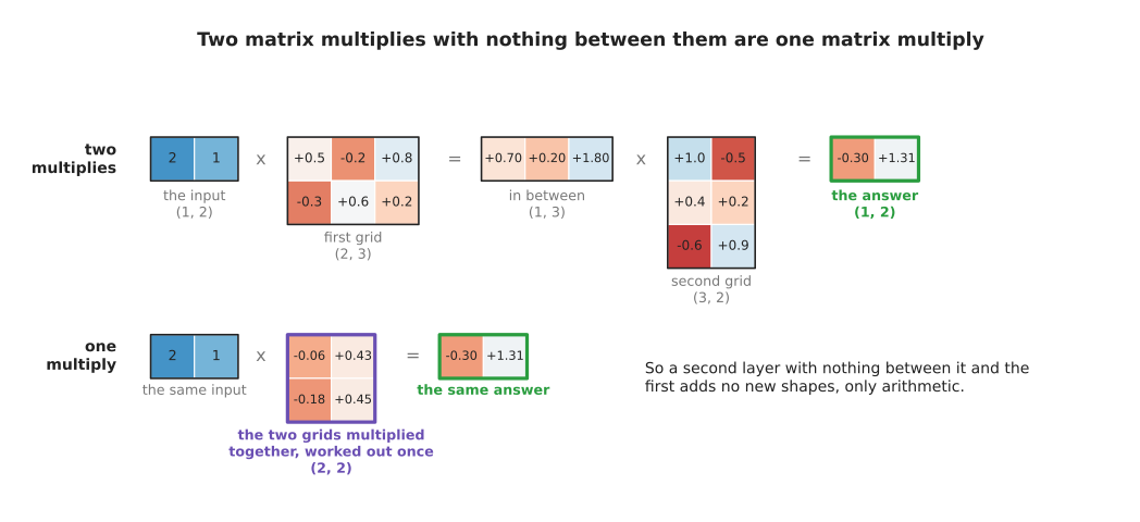
Two matrix multiplies with nothing between them give exactly the answer that one multiply by the product of the two grids gives, so depth on its own buys nothing.
Because that replacement is always possible, depth on its own buys nothing. A stack of ten matrix multiplies can still only do what one matrix multiply does. So everything a network can do beyond drawing a straight line comes from the rule applied between the layers. That rule is the non-linearity, and the ReLU is the simplest one in common use.
Before adding a ReLU, it helps to see how badly a straight line does on its own. The picture below fits the best possible straight line to a curve that bends.
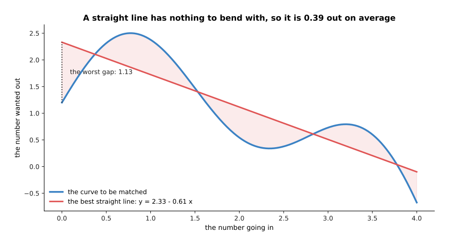
The best straight line through a curve that bends is 0.39 away from it on average and 1.13 away at its worst.
The blue curve there is made up. It stands for any relationship between one measured number and one wanted number that is not a straight line. The best straight line through it is y = 2.33 - 0.61 x. That line sits 0.39 away from the curve on average and 1.13 away at its worst, which happens at the left-hand end. No choice of two numbers does better, because two numbers is all a straight line has.
Now put one ReLU neuron beside that line. Its output is 0 until the total inside it passes 0, and after that it rises straight. The picture below draws that shape.
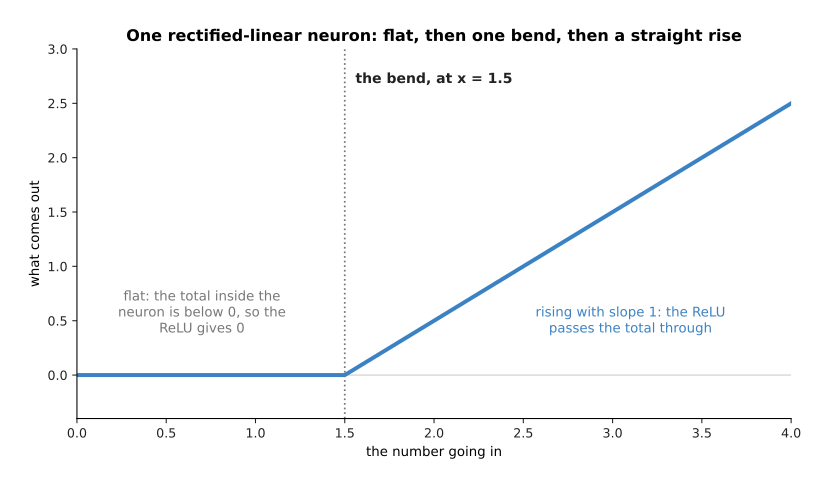
One rectified-linear neuron gives a flat part and then a straight rise, and the place where the two meet is the bend.
In that picture the turn happens at x = 1.5, because that is where the total inside the neuron passes 0. The weight and bias of the neuron decide where the turn happens. The weight that the next layer puts on the neuron decides something different, and the picture below shows what.
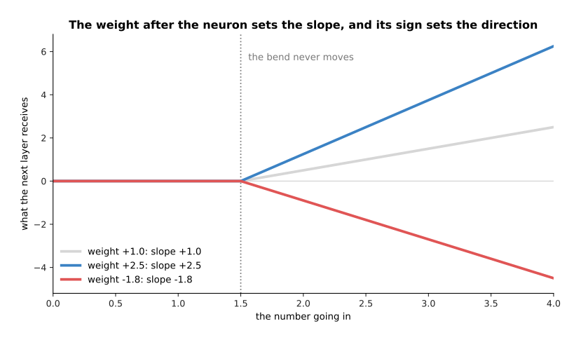
The weight in the layer after the neuron scales the whole shape, so it sets how steep the rising part is, and its sign decides whether the shape rises or falls.
A weight of 2.5 makes the rising part two and a half times as steep. A weight of -1.8 makes it fall instead of rise. The bend itself does not move, because the next layer's weight cannot change where the total inside the neuron passes 0. Now add two such neurons to a straight line, and the result is a line in three pieces.
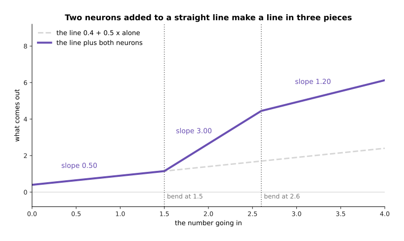
Adding two rectified-linear neurons to a straight line gives a line in three pieces, with slopes 0.50, then 3.00, then 1.20.
So one neuron buys exactly one bend. The next question is what those bends do to the gap between the red line and the blue curve. The picture below adds them one at a time.
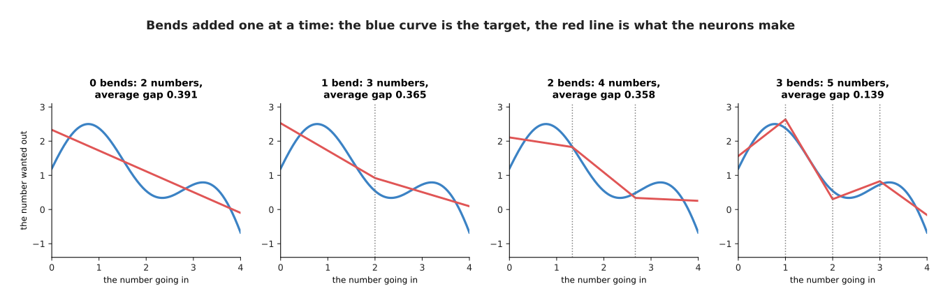
Bends added one at a time, each one costing one neuron and shrinking the gap between the red line and the blue curve.
The gap closes, but it does not close evenly. With no bends the gap is 0.391. With one bend placed in the middle it is 0.365. With two bends it is 0.358. With three bends it drops to 0.139. The first two bends barely help, because they are in the wrong places. That is worth noticing rather than hiding, because where the bends go is one of the things training has to find out. Since each neuron buys one bend, the next section asks what a great many bends buy.
2. Enough bends will follow any shape#
The section before showed that one neuron buys exactly one bend, so this section adds many neurons and measures the fit. The answer is the property that makes neural networks worth using at all.
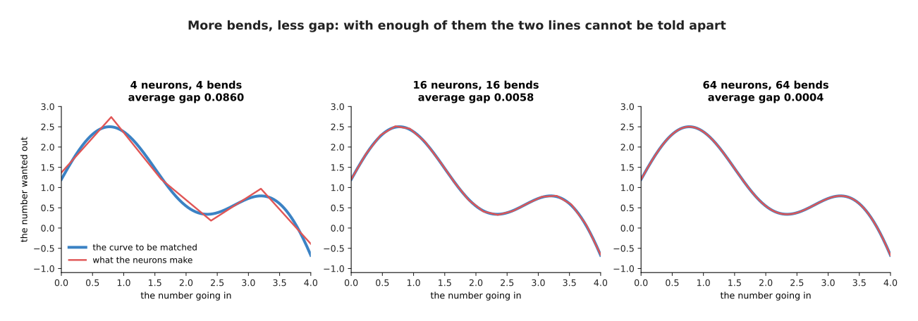
With 4 bends the red line is visibly straight between the turns, with 16 it is hard to see the difference, and with 64 the two lines cannot be told apart.
Four neurons leave the gap at 0.0860, and the red line is visibly made of straight pieces. Sixteen neurons bring the gap to 0.0058, which is already hard to see. Sixty four neurons bring it to 0.0004, and at that point the red line and the blue curve cannot be told apart on the page. Nothing about the curve was used in choosing where the bends went. Only their number changed.
The plot below puts those numbers on one scale, so the pattern in them is visible.
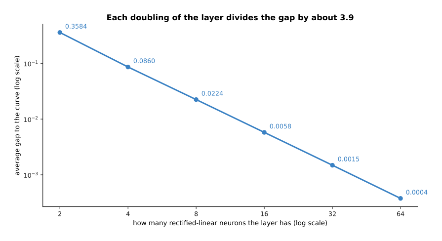
Each doubling of the layer divides the average gap by about 3.9, which is why a modest number of neurons is usually enough.
The gap runs 0.358, 0.0860, 0.0224, 0.0058, 0.0015 and 0.0004 as the layer grows from 2 neurons to 64. So each doubling of the layer divides the gap by about 3.9. A relationship of that kind is the practical form of a result that mathematicians proved in the late 1980s. That result says that a single layer of enough neurons, with a non-linear rule, can come as close as you like to any smooth shape. However, the result says nothing about how many neurons "enough" is, and nothing about how to find their weights. That is why it is reassuring rather than useful.
Where the bends sit matters as much as how many of them there are. The two plots below show the same three neurons with their bends in two different places.
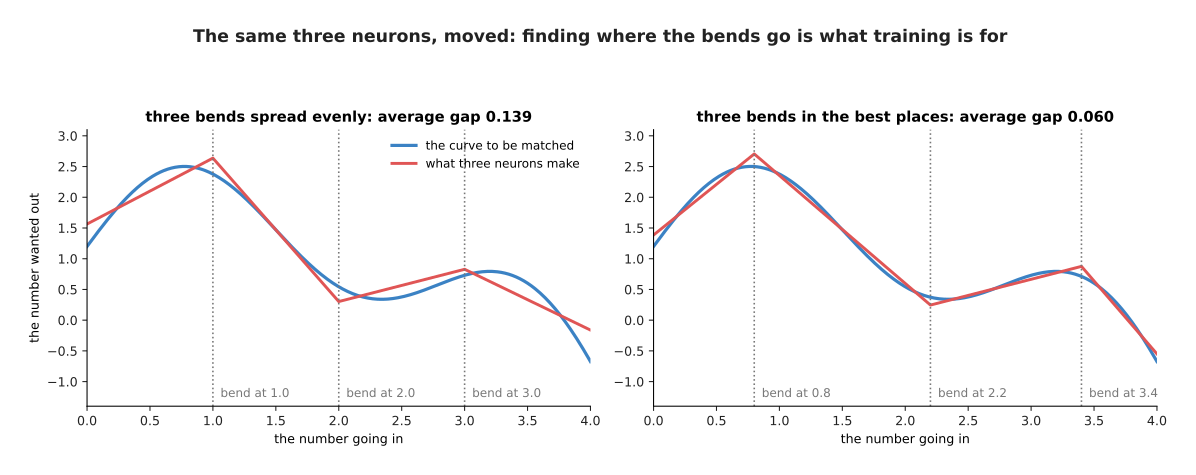
The same three neurons, with their bends moved: putting them at 0.8, 2.2 and 3.4 instead of 1.0, 2.0 and 3.0 more than halves the gap.
Three bends spread evenly at 1.0, 2.0 and 3.0 leave a gap of 0.139. The best three places are 0.8, 2.2 and 3.4, and they leave a gap of 0.060. So the same three neurons are 2.3 times closer to the curve for no extra cost. In the fits on this page the places of the bends were either spread evenly or found by trying every combination. Only the weights after the bends were worked out properly, by solving a small system of equations. A real network does something quite different. In a real network the bend of each neuron moves as that neuron's own weight and bias change, so training adjusts how many bends there are and where every one of them sits at the same time. More bends always closed the gap here, so the next section asks whether more neurons are always better.
3. Capacity: too little, about right, and too much#
The section before showed that enough bends will follow any shape, so more neurons means a smaller gap. That sounds like an argument for always using more neurons. This section comes now to make the argument against, and it starts with two words that the rest of the book uses constantly.
The parameter count of a network is simply how many weights and biases it holds. It follows from the widths and the number of layers by plain arithmetic, so there is nothing to estimate. The capacity of a network is how complicated a relationship it can express. For the one-input networks on this page capacity has an exact meaning, because a layer of W rectified-linear neurons gives a line of W bends and no more.
The table below counts parameters for nine networks. Read it one row at a time. Each row is one width of hidden layer, and the three columns are one, three and eight hidden layers.
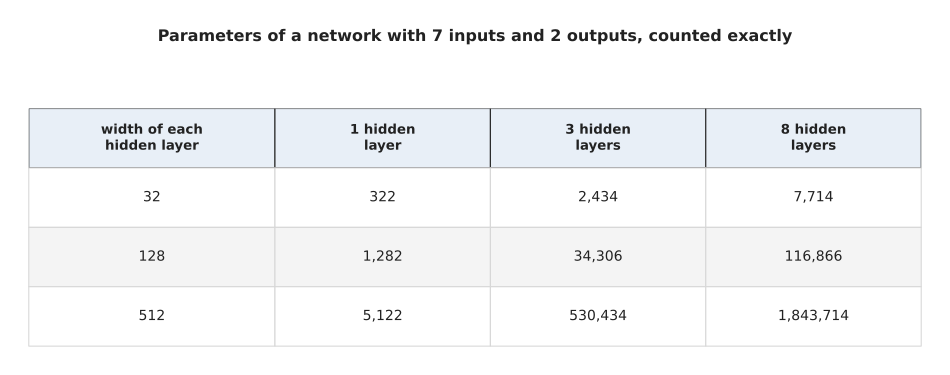
Parameter count follows from the widths and the number of layers, with nothing to guess.
A network with 7 inputs, 2 outputs and one hidden layer of 32 neurons holds 322 parameters. Three hidden layers of 32 hold 2,434, and eight hold 7,714. Now widen the hidden layers to 512. One such layer holds 5,122, three hold 530,434 and eight hold 1,843,714. So width costs more than depth. The reason is that joining two layers of width W takes W x W weights, so doubling the width roughly quadruples the cost of every join.
Cost and capacity rise together, but not at the same rate. The plot below draws both for a network with one input.
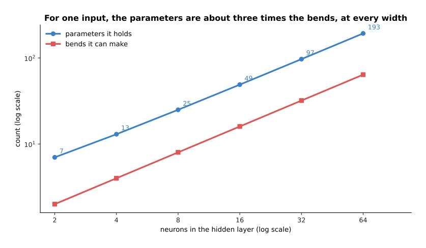
For a network with one input, the parameter count is about three times the number of bends at every width: 16 neurons hold 49 parameters and make 16 bends, and 64 neurons hold 193 and make 64.
So paying three parameters buys roughly one bend. The question this section asks is whether buying more bends is always worth it. To answer that, give a network readings of the curve instead of the curve itself, because readings are what a real problem offers.
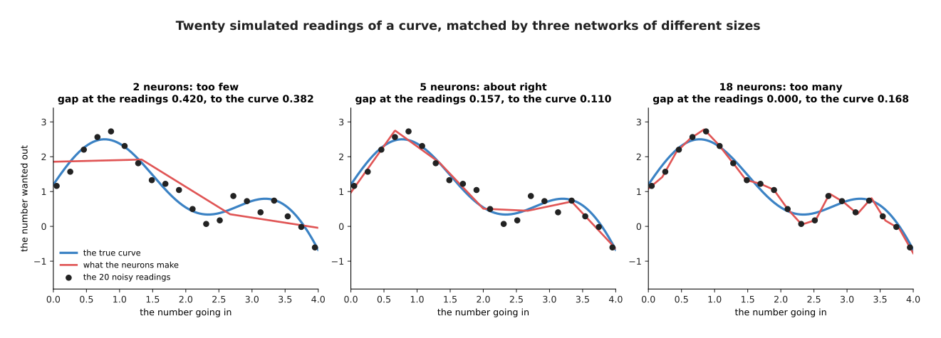
Twenty simulated readings of the curve, matched by three networks: too few neurons cannot follow the curve, enough neurons follow it well, and too many follow the measurement errors instead.
The twenty black dots in that picture are simulated. They were taken at even steps along the made-up curve, with a random error added to each one, which is what a real measurement looks like. With 2 neurons the red line is 0.420 away from the readings and 0.382 away from the true curve, because it cannot bend enough to follow either. With 5 neurons it is 0.157 away from the readings and 0.110 away from the curve, which is the best of the three. With 18 neurons it passes exactly through all twenty readings, so its gap at the readings is 0.000. Yet its gap to the true curve has risen to 0.168. The reason is that between the readings it has followed the measurement errors rather than the shape underneath them.
Those two measurements part company at a particular width, and the plot below shows where.
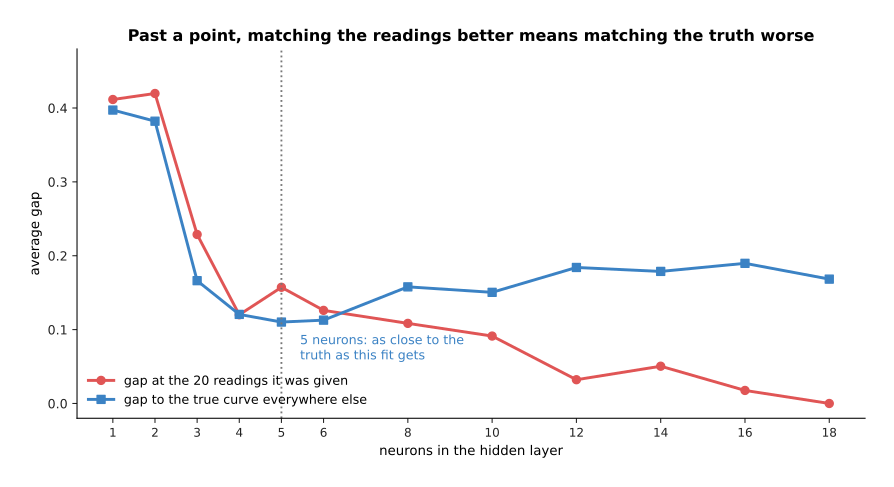
Past five neurons, every extra neuron brings the line closer to the readings it was given and no closer to the truth.
The gap at the readings falls steadily, from 0.41 at one neuron to 0.000 at eighteen, because more bends can always be made to pass nearer the dots. The gap to the true curve falls only to 0.110 at five neurons, and after that it climbs back, reaching 0.190 at sixteen neurons. The word for what happens on the right-hand side of that plot is overfitting. Overfitting is the subject of overfitting and generalisation, which also explains why the honest way to measure a model is on readings it has never seen. For this page the lesson is narrower. Capacity is something to choose, and not something to maximise. The next section asks what that choice costs when the input is a photo, because the parameter count of a fully connected layer grows with the number of inputs.
4. Why a fully connected layer is the wrong shape for a photo#
The sections from one bend per neuron to choosing capacity used one input number, which kept the pictures simple. A camera gives 150,528 input numbers instead. This section comes now to apply the parameter count of the section before to an input of that size. At that size the fully connected layer of layers and depth stops being a sensible choice, for two separate reasons. The first reason is about counting, and the second is about position.
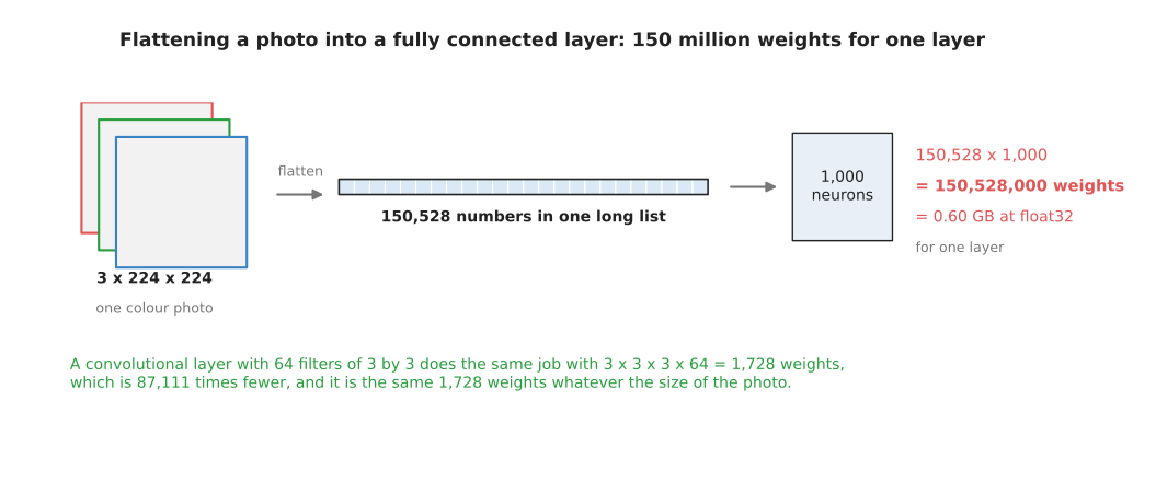
One fully connected layer of 1,000 neurons on one colour photo needs 150,528,000 weights, which is 0.60 gigabytes at four bytes each.
Count the first reason. A colour photo of 224 rows by 224 columns is 3 x 224 x 224 = 150,528 numbers. A fully connected layer joins every input to every neuron, so 1,000 neurons need 150,528 x 1,000 = 150,528,000 weights. At four bytes a weight that is 0.60 gigabytes, for one layer. A convolutional layer with 64 filters of 3 by 3, which the next section explains, does the same job with 3 x 3 x 3 x 64 = 1,728 weights. That is 87,111 times fewer.
The counting gets worse as the picture gets larger, and this is the part that makes the fully connected layer hopeless rather than merely expensive.
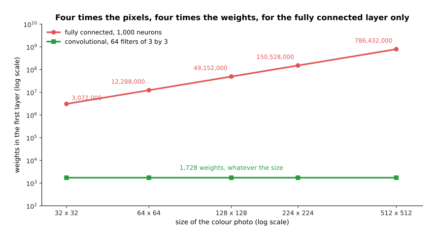
Four times the pixels means four times the weights for the fully connected layer, and no change at all for the convolutional one.
At 32 by 32 the fully connected layer needs 3,072,000 weights. At 128 by 128 it needs 49,152,000. At 224 by 224 it needs 150,528,000. At 512 by 512 it needs 786,432,000. The 64 filters need 1,728 weights at every one of those sizes, because the same filter is used at every position in the picture.
The second reason is position, and it is the deeper of the two. Flattening a picture into a list throws away which numbers were next to each other. So to a fully connected layer, one pixel and the pixel beside it are no more related than any two numbers in the list. The picture below shows what that costs.
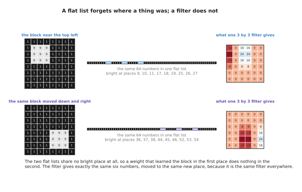
Moved three rows down and three columns right, the block lights up a completely different set of places in the flat list, while the filter gives exactly the same numbers in a new place.
In that drawing the same bright 3 by 3 block sits near the top left in one row, and three rows down and three columns right in the other row. In the flat list the first block lights up places 9, 10, 11, 17, 18, 19, 25, 26 and 27. The second lights up places 36, 37, 38, 44, 45, 46, 52, 53 and 54. Those two sets share no place at all. So a weight that learned to recognise the block in the first position does nothing whatever in the second position. The network therefore has to learn the same thing again for every position the block might appear in. The filter in the right-hand column behaves differently. It gives exactly the same six numbers in both rows, simply moved to a new place. The next section asks what that filter actually computes, because it is the layer that solves both the counting problem and the position problem.
5. The convolution, worked out number by number#
The section before showed why a fully connected layer is the wrong shape for a photo, and it named a layer that fixes both problems without saying what that layer does. So this section works it out in full. A convolution slides a small grid of weights over a larger grid of numbers. At every position it multiplies each number under the small grid by the weight on top of it, and then adds the results together. That total is one number of the answer. The small grid of weights is called a filter, and a filter is a detector for one small pattern.
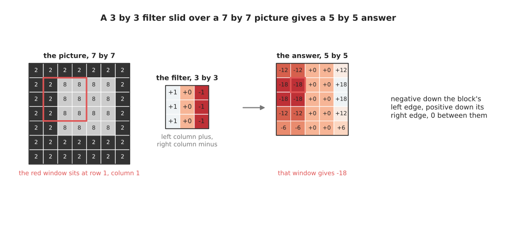
A 3 by 3 filter slid over a 7 by 7 picture gives a 5 by 5 answer, with -18 where the window sits on the left edge of the bright block and +18 where it sits on the right edge.
The picture there is made up. It is a dark table of 2s with a bright block of 8s lying on it. The filter has +1 down its left column, 0 down its middle column and -1 down its right column, so it asks whether the left side of its window is brighter than the right side. The answer grid is negative down the left edge of the block and positive down its right edge. It is exactly 0 in the two middle columns, because there the window sees the same brightness on both of its sides. The largest answers, -18 and +18, appear where the whole window straddles an edge. Smaller answers such as -12 and -6 appear where only part of the window covers the edge. So this filter is a detector for the boundary between dark and bright.
The picture below works three of those positions out multiply by multiply.
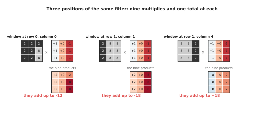
Three positions of the same filter: nine multiplies and one total at each, giving -12, -18 and +18.
Follow the three positions one at a time. At row 0 and column 0 the window covers mostly table, with two 8s at its right. The nine products are therefore +2, 0, -2, +2, 0, -8, +2, 0 and -8, which add to -12. At row 1 and column 1 the window straddles the left edge of the block, giving +2, 0 and -8 three times over, which adds to -18. At row 1 and column 4 the window straddles the right edge, giving +8, 0 and -2 three times over, which adds to +18. So the sign of the answer tells you which way the brightness changes, and the size of the answer tells you how sharply it changes.
A convolutional layer has many filters, not one, and each filter detects something different. The picture below runs two filters over the same picture.
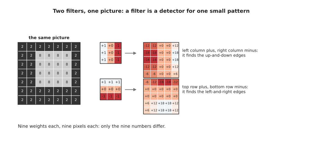
Two filters, one picture: changing only the nine numbers in the filter changes which pattern it finds.
The second filter there has +1 along its top row and -1 along its bottom row. So it finds the edges that run left and right, instead of the edges that run up and down. On the same picture it gives -18 along the top of the block and +18 along the bottom, in the very places where the first filter gave 0. Both filters have nine weights, and both look at nine pixels at a time. The only difference between them is the nine numbers they hold. On this page those numbers were chosen by hand, to make the arithmetic clear. In a real network every one of them is found during training, which is how the network decides for itself which patterns are worth detecting.
Three choices decide how big the answer is, and the picture below shows all three on the same picture and filter.
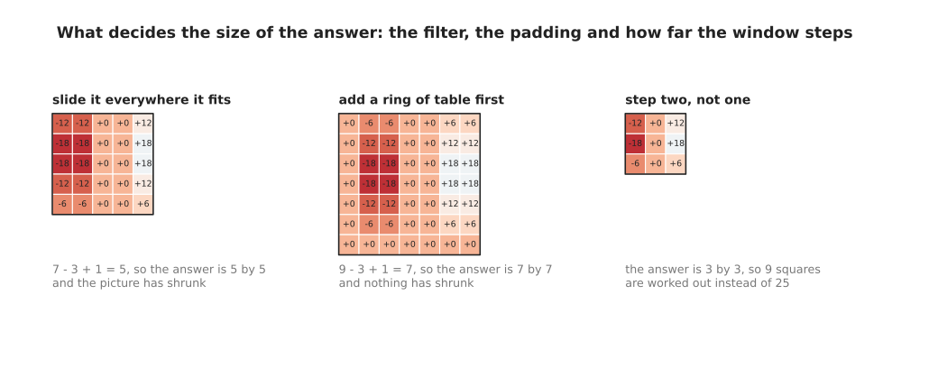
What decides the size of the answer: the size of the filter, whether a ring is added round the picture first, and how far the window steps each time.
The first choice is to slide the window everywhere it fits. That gives 7 - 3 + 1 = 5, so the answer is 5 by 5 and the picture has shrunk by one pixel on each side. The second choice is to add a ring of table round the picture before sliding, which is called padding. That gives 9 - 3 + 1 = 7, so nothing shrinks. The third choice is to move the window two places at a time instead of one, which is called the stride. That gives a 3 by 3 answer here, so 9 squares are worked out instead of 25. On a large picture a stride of two gives about a quarter of the squares and therefore about a quarter of the arithmetic, because it halves the answer in both directions. Those three choices appear in every convolutional layer anyone writes. One layer sees only a 3 by 3 window, so the next section asks what a stack of such layers can see.
6. The convolutional neural network, and where it still earns its place#
The section before worked out one convolution, number by number. This section stacks those layers, because one window is far smaller than any object in a photo. A network built mainly from such layers is called a convolutional neural network, which is often shortened to CNN. Stacking those layers is what turns a detector of edges into a detector of objects. The reason is that each layer looks at the answers of the layer before it, rather than at the picture itself.
How far back into the picture one number can see is worth counting, because it decides whether the network can relate two things that are far apart. The picture below counts it for five layers of 3 by 3 filters.
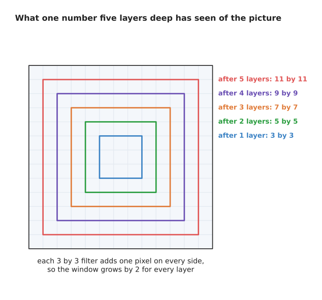
With 3 by 3 filters that step one place at a time, the window on the picture grows by 2 pixels each layer, so one number after five layers has seen 11 by 11 pixels.
Growing by 2 pixels a layer is slow. Covering a 224 pixel picture that way would take 112 layers, which no one builds. Making every second layer step two places instead of one changes the arithmetic completely, and the plot below compares the two.
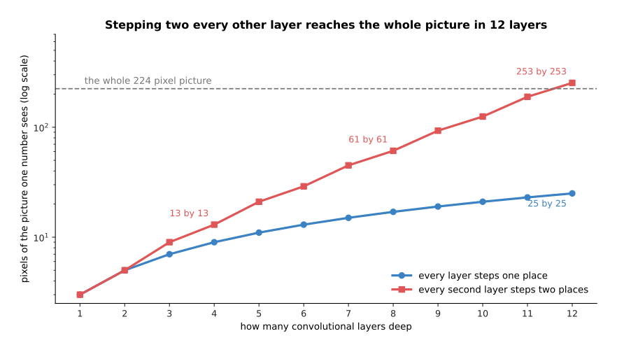
Stepping two places every second layer reaches 13 by 13 pixels after four layers, 61 by 61 after eight and 253 by 253 after twelve, while stepping one place every layer reaches only 25 by 25 after twelve.
That is why real convolutional networks shrink the grid as they go. The picture below shows what that shrinking looks like across four stages.
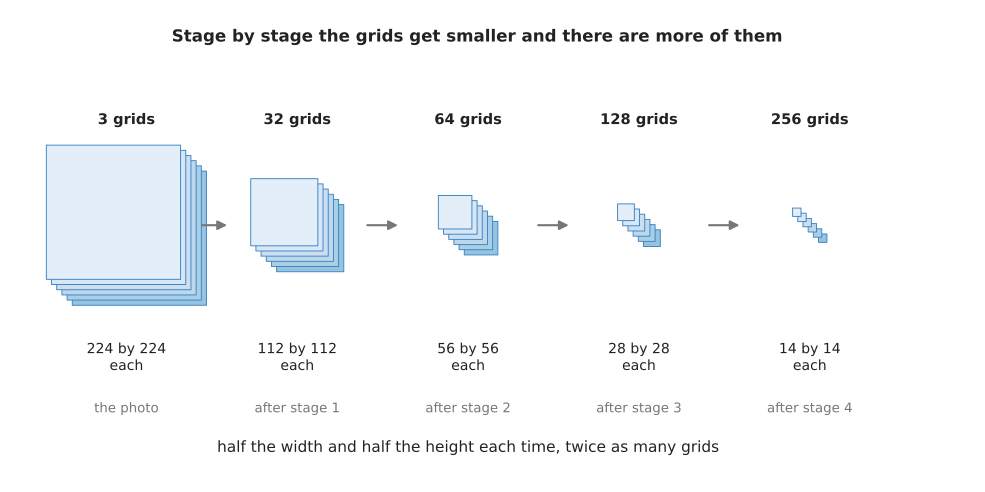
Each stage halves the width and the height of the grid and doubles the number of grids, so a photo of 3 grids of 224 by 224 becomes 256 grids of 14 by 14.
The table below gives the same four stages with their exact costs. Read it one row at a time. Each row is one stage, and the columns give the shape that comes out, the weights that stage holds, and the arithmetic it does for one photo.
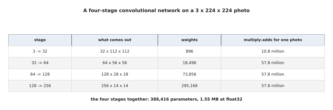
Four stages of 3 by 3 filters that halve the grid each time, with the shape, the weight count and the arithmetic of each.
The first stage turns the photo's 3 colour grids into 32 grids of 112 by 112, using 896 weights. The second gives 64 grids of 56 by 56, using 18,496 weights. The third gives 128 grids of 28 by 28, using 73,856. The fourth gives 256 grids of 14 by 14, using 295,168. The four stages together hold 388,416 parameters, which is 1.55 megabytes. The pattern is that the grids get smaller while the number of grids grows, and that is the usual shape of a picture network.
Now set that whole stack against the one fully connected layer that a photo made so costly. The two charts below compare them, first on the weights they hold and then on the arithmetic they do.
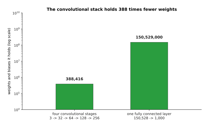
The whole convolutional stack holds 388,416 weights, which is 388 times fewer than the 150,529,000 of one fully connected layer.
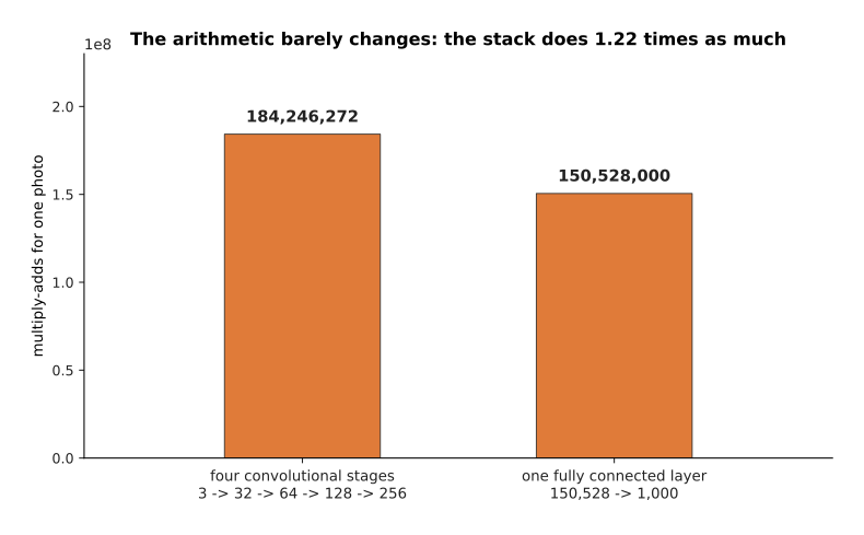
The arithmetic barely changes between the two: the convolutional stack does 1.22 times as many multiply-adds as the fully connected layer.
So the convolutional stack has 388 times fewer weights and does about a fifth more arithmetic. That is exactly the bargain you want. Weights are what must be stored, carried to the robot and learned from examples, so having fewer of them helps three times over. Arithmetic is what the hardware of the previous page is good at, so having a little more of it costs almost nothing.
So where do convolutional networks stand now? They are still the right choice when a model must run many times a second on the computer that the robot carries. The reason is that they are small, and their arithmetic suits modest hardware. They are also still common for depth maps and for small pictures. They survive inside models that are called something else as well, and the picture below shows the clearest example.
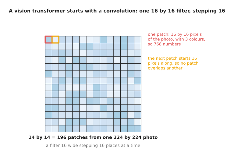
A vision transformer begins by cutting a 224 by 224 photo into 196 patches of 16 by 16 pixels, and that first step is one convolution with a 16 by 16 filter and a stride of 16.
What convolutional networks lost is the top end. A convolution can only relate things that fall inside one window. So relating two distant parts of a picture takes many layers, as the reach plot above showed. Attention relates every part of a picture to every other part in one step, and it also trains better on very large collections of pictures. That is why large vision models, and every model that joins pictures with language, are now built from transformers. What attention actually computes is worked out with real numbers in attention.
The cost of that change is real. A transformer needs more examples than a convolutional network to reach the same accuracy on pictures, because it starts with no built-in idea that nearby pixels belong together. Its arithmetic also grows with the square of the number of patches, so doubling the patches along each side multiplies the work by sixteen.
Every fit on this page was already good, so the reading below starts with how a network finds its weights.
7. Where to read next#
- Questions and answers is the next page, and it closes the chapter by answering the questions the other pages raised without stopping for, such as how many layers to use and where the weights come from.
- The score of being wrong opens the next chapter, giving the number that says how wrong an answer is, which this page kept calling the gap.
- Gradient descent then explains how the weights and the bends that each neuron buys are actually found, instead of being solved for or tried one by one.
- Overfitting and generalisation takes capacity, too little and too much further and says how to tell honestly whether a model has too much capacity.
- Attention is the operation that replaced the convolution at the top end of vision, worked out with real numbers.
- Vision backbones compares convolutional and transformer backbones for pictures and says where each still wins.
- Image classification is the catalogue page for the simplest job a convolutional network does on a robot, with the named models that do it.
8. Using it in Python#
The layers on this page are a line each in PyTorch, and the parameter counts it printed are counts you can check yourself. Every number in a comment below is what the line really prints.
import torch
from torch import nn
from torch.nn import functional as F

# bends: one hidden layer of ReLU neurons, one bend for each neuron
net = nn.Sequential(nn.Linear(1, 16), nn.ReLU(), nn.Linear(16, 1))
print(sum(p.numel() for p in net.parameters()))   # 49 parameters, 16 bends

# the wrong shape for a photo: the two choices of first layer for one colour photo
photo = torch.zeros(1, 3, 224, 224)
dense = nn.Linear(3 * 224 * 224, 1000)
print(sum(p.numel() for p in dense.parameters()))  # 150529000
conv = nn.Conv2d(in_channels=3, out_channels=64, kernel_size=3, padding=1)
print(sum(p.numel() for p in conv.parameters()))   # 1792
print(conv(photo).shape)                           # torch.Size([1, 64, 224, 224])

# the convolution: the worked example, with the filter set by hand instead of learned
grid = torch.full((1, 1, 7, 7), 2.0)
grid[0, 0, 1:5, 2:6] = 8.0
edge = torch.tensor([[1.0, 0.0, -1.0]] * 3).reshape(1, 1, 3, 3)
answer = F.conv2d(grid, edge)
print(answer.shape)                                # torch.Size([1, 1, 5, 5])
print(answer[0, 0, 1])                             # tensor([-18., -18., 0., 0., 18.])

# the size of the answer: padding keeps the size, a stride of two shrinks it further
print(F.conv2d(grid, edge, padding=1).shape)       # torch.Size([1, 1, 7, 7])
print(F.conv2d(grid, edge, stride=2).shape)        # torch.Size([1, 1, 3, 3])
The library gives you the layers and the arithmetic. It also starts every weight at a
small random number, so that the neurons differ from one another from the beginning.
nn.Conv2d holds the filters, does the sliding at whatever speed the card allows, and
takes the padding and the stride of
the worked convolution as ordinary
arguments.
One small honesty is worth stating. What the libraries call a convolution does not flip the filter, although the mathematical operation of that name does. So what they compute is strictly a cross-correlation. Nothing changes because of this, since the filter's numbers are learned either way round.
What you still decide is everything the section on capacity was about. You choose the width and the depth, which together fix the parameter count and therefore the capacity, and that section showed that more is not better. You choose the filter size, the stride and the padding, which fix how fast the grid shrinks and how far one late number can see, as the count of stacked convolutions showed. You also choose whether a convolution is the right layer at all. For a small fast model on a robot it usually is. For a large model that must relate distant parts of a picture it usually is not.