This page explains the pinhole camera model as a technique you can use in any program, and it answers four questions. How does a camera turn a point in the room into a pixel? How do you turn a pixel and a depth reading back into a point? How many millimetres does one pixel cover? And how do you find a point when the camera gives no depth at all?
It is for a reader who has read Book 2's cameras: the basics, which explains pixels, focal length and the four lens numbers from the start, and finding one box, which works through one pixel slowly. This page does not repeat those explanations, but instead collects the formulas into one method, adds the parts those pages leave out, and shows where the method is used on an arm.
Contents#
- The idea in one sentence
- How it works · Projection: a point to a pixel · The same rule as one matrix · Back-projection: a pixel and a depth to a point · A whole depth picture at once · Pixels to millimetres · No depth: where a pixel's ray meets a known plane · Lens distortion: where the pinhole stops being true · Pseudocode
- Where it is used on a robot arm
- Where it works, and where it does not
- Libraries that provide it
- Why this model, and what it costs
- The learned alternative
- Where to read next
- Using it in Python
1. The idea in one sentence#
Every pixel looks out from one point along one straight line, and a camera records only which line, never how far along it.
The one point is called the pinhole, or the camera's optical centre, and in a real camera it is the middle of the lens. The straight line through the pinhole and a pixel is called that pixel's ray. Here is an everyday example. Hold up a finger at arm's length, close one eye, and line the finger up with a distant tree. Both the finger and the tree then lie on the same line from your eye, so they land on the same spot in your eye and your one eye cannot tell which is nearer. A camera has the same limit, and the pinhole model is the arithmetic of that line.
So the picture below shows two rays out of a pinhole, drawn from the side.
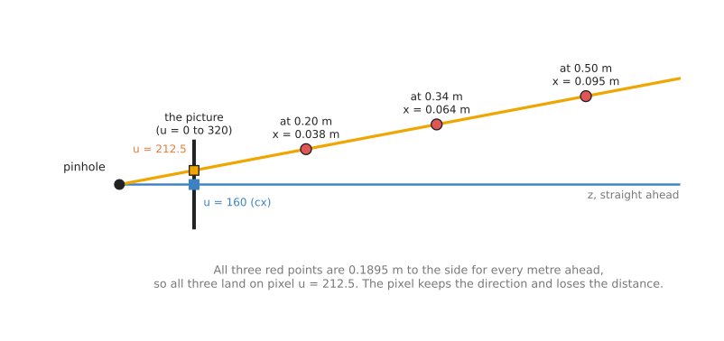
The blue ray goes straight ahead and lands on the middle of the picture, at pixel u = 160, while the orange ray lands on pixel u = 212.5. The three red points sit on that orange ray at 0.20 m, 0.34 m and 0.50 m ahead, so they are different points in the room, but all three land on the same pixel.
2. How it works#
Section 1 said in words what a camera records, so this section writes the same thing as arithmetic. The whole model is two formulas, one for each direction, and this section writes them out, puts them in matrix form, and then adds the practical pieces around them.
Every number on this page uses Book 2's simulated camera, whose picture is 320 ×
240 pixels. Its four lens numbers are fx = fy = 277.1 pixels, cx = 160 and
cy = 120, and it hangs 0.40 m above the middle of a table and looks straight
down. The numbers were checked by running the formulas in Python.
Projection: a point to a pixel#
Projection takes a point measured from the camera and gives the pixel it
lands on. The camera's axes follow the picture, so x points right, y points
down, and z points straight out of the lens, and this frame is called the
camera's optical frame.
u = fx · (x / z) + cx
v = fy · (y / z) + cy
In other words, divide the sideways distance by the distance ahead, multiply by the focal length in pixels, and add the position of the middle of the picture.
For example, take the spot on top of the red box from Book 2, which is at x =
0.06442 m, y = -0.04110 m and z = 0.340 m from the camera.
u = 277.1 · (0.06442 / 0.340) + 160 = 277.1 · 0.18946 + 160 = 212.5
v = 277.1 · (-0.04110 / 0.340) + 120 = 277.1 · -0.12089 + 120 = 86.5
So the spot lands on pixel (212.5, 86.5). Now double all three distances, to
(0.12884, -0.08220, 0.680), and the ratios x / z and y / z do not change, so
the pixel does not change either. That is the ray from the picture above,
written as arithmetic, and the division by z is exactly where the distance is
lost.
The same rule as one matrix#
Libraries store the four lens numbers as a 3 × 3 grid called the intrinsic
matrix, written K. Book 2 shows it arriving in ROS's CameraInfo message,
in
k in detail.
      [ fx   0   cx ]   [ 277.1    0    160 ]
K  =  [  0  fy   cy ] = [   0    277.1  120 ]
      [  0   0    1 ]   [   0      0      1 ]
Projection is then one multiplication followed by one division. That means you
multiply K by the point to get three numbers, and then divide the first two by
the third.
K · (0.06442, -0.04110, 0.340) = (72.25, 29.41, 0.340)
pixel = (72.25 / 0.340, 29.41 / 0.340) = (212.5, 86.5)
The third number is the depth, so the division by it is the step that loses
distance. You will see this form in every library, and in papers, where it is
often written with a scale factor: s · (u, v, 1) = K · (x, y, z), with s
equal to z.
Back-projection: a pixel and a depth to a point#
Back-projection runs the formula the other way, and it is also called deprojection, which is the word Book 2 uses. However, it needs one extra number, which is the depth reading for that pixel from a depth camera.
x = (u - cx) · depth / fx
y = (v - cy) · depth / fy
z = depth
For pixel (212.5, 86.5) with a depth of 0.340 m:
x = (212.5 - 160) · 0.340 / 277.1 =  52.5 · 0.0012270 =  0.06442 m
y = ( 86.5 - 120) · 0.340 / 277.1 = -33.5 · 0.0012270 = -0.04110 m
z = 0.340 m
That is the point we started from, so the two formulas undo each other exactly. Book 2 walks through the same four steps with pictures of the two similar triangles in pixel plus depth gives back the point.
However, two details decide whether the answer is right in practice.
First, the depth must be the distance straight ahead, along z, not the
distance along the slanted ray. Nearly every depth camera reports it this way,
and
depth is not distance
explains why. If a sensor reports the slanted distance instead, divide it by the
length of the ray direction ((u - cx) / fx, (v - cy) / fy, 1) first. For our
pixel that length is 1.0249, so a slanted reading of 0.3485 m becomes a depth of
0.340 m.
Second, u and v should be the middle of the pixel, because pixel number 212
covers the strip from 212 to 213 and its middle is therefore 212.5. Using 212
instead moves the point by half a pixel, which is 0.61 mm at this depth.
A whole depth picture at once#
Because a depth camera gives a depth for every pixel, back-projecting all of them gives a point cloud, which is a list of 3D points, one per pixel. Book 2's camera makes 76,800 points from one picture.
For example, the picture below shows one row of pixels, v = 120, across the
table and the red box. On the left is what the camera gives, which is one depth
per pixel, and on the right is what back-projection makes, which is one point
per pixel placed along its ray.
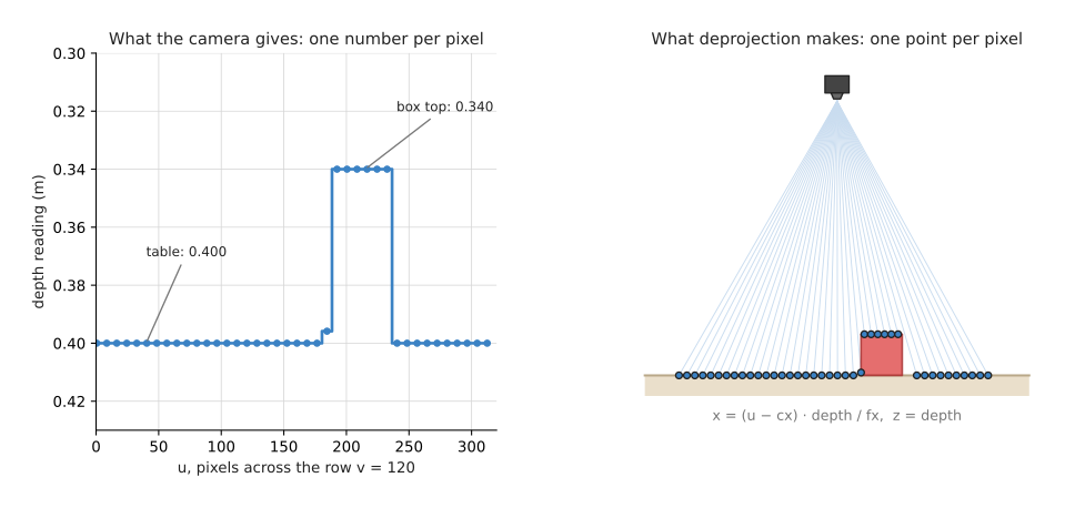
The picture draws every eighth pixel, and the table pixels read 0.400 m while the box-top pixels read 0.340 m. Just to the left of the box, one drawn pixel sees the box's side and reads 0.396 m, in between. To the right of the box there is a gap in the points, because the box hides that strip of table from the camera, so no pixel ever looks at it. This missing strip is called a shadow, and every point cloud from one camera has them.
However, in a program you rarely loop over pixels one at a time. Instead, you
compute the x and y factors once for every pixel, (u - cx) / fx and (v - cy) / fy, and multiply the whole depth picture by them in one step. The factors
never change while the camera and resolution stay the same, so they can be
stored.
Pixels to millimetres#
Back-projection also tells you how much of the world one pixel covers. At depth
z, moving one pixel to the side moves the point by z / fx metres.
one pixel covers = depth / fx
at 0.340 m: 0.340 / 277.1 = 0.001227 m = 1.227 mm
at 0.400 m: 0.400 / 277.1 = 0.001444 m = 1.444 mm
This is the most useful single number for judging whether a camera can do a job. If a gap you must measure is 1 mm wide, and one pixel covers 1.4 mm, no program can measure it. So the chart below shows the number against depth for Book 2's camera, and for the same lens on a sensor with twice the pixels across.
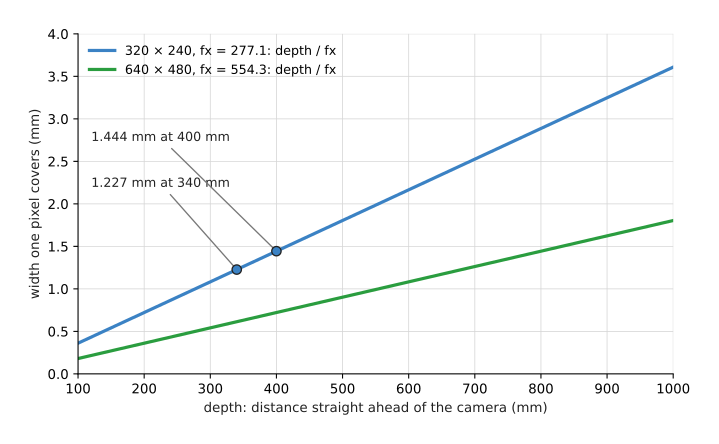
Both lines are straight, because the width grows in proportion to depth, and doubling the resolution halves the width at every depth. Book 2 explains the trade between field of view and resolution in field of view and resolution are separate knobs.
The same rule also measures size. The red box's top is 6 cm wide, so at 0.340 m
it covers 0.060 / 0.001227 = 48.9 pixels. Read the other way, a box 48.9
pixels wide at 0.340 m is 6 cm wide.
No depth: where a pixel's ray meets a known plane#
A colour-only camera gives no depth, but if you know the surface the object lies on, you can still find the point. The ray from the pixel is known and the plane of the table is known, so the point is where the two meet. Book 2 calls this knowing the surface the object sits on.
So the method has three steps, which turn the pixel into a ray and then follow that ray down to the table.
- Turn the pixel into a ray direction in the camera's frame:
d = ((u - cx) / fx, (v - cy) / fy, 1). - Turn that direction into the room's frame with the camera's rotation, which the
rigid transforms page explains. The ray now starts at
the camera's position
cand runs along the turned directiond'. - Find how far along the ray the table is. For a table at height 0, the point is
c + t · d', wheret = -c_z / d'_z. Becausedhad a 1 in itszplace,tis also the depth that pixel would have read.
For example, the picture below uses a tilted camera, which is the usual case on a wrist. The camera is 0.40 m above the table and 0.20 m back from its middle, looking forward and 60° down.
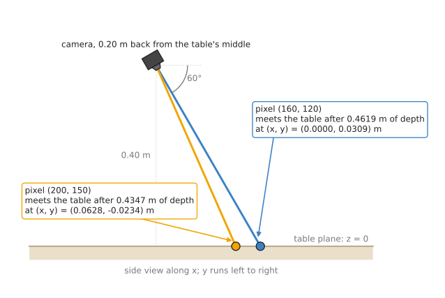
The middle pixel (160, 120) looks straight along the camera's axis, and its ray meets the table after a depth of 0.4619 m, at (0.0000, 0.0309) m in the room. Then pixel (200, 150) meets the table after 0.4347 m, at (0.0628, -0.0234) m. Neither number came from a depth sensor, because both came from the pixel, the lens numbers, the camera's pose, and the fact that the table is flat.
However, the method breaks the moment the object is not on the plane you assumed. For example, a pixel on top of a box 6 cm tall would give a point on the table behind the box instead.
Lens distortion: where the pinhole stops being true#
A real lens bends light a little, so straight lines in the room come out slightly curved in the picture. The pinhole model assumes no bending, so real programs correct the bending first and then use the pinhole formulas on the corrected pixels, and that correction step is called undistortion.
This bending is described by a few more numbers, usually five, called the distortion coefficients. They are measured by calibration, which also shows how large the bending can be: several pixels near the corners of a wide lens. Book 2's simulated camera has no bending at all, so its five distortion numbers are zero.
Pseudocode#
Here is the whole technique in plain steps, and it works in any language.
lens numbers: fx, fy, cx, cy

project(point):                       # a point in the camera frame to a pixel
    if point.z <= 0: return nothing   # behind the camera, or on it
    u = fx * point.x / point.z + cx
    v = fy * point.y / point.z + cy
    return (u, v)

back_project(u, v, depth):            # a pixel and a depth to a point
    if depth is missing or depth <= 0: return nothing
    x = (u - cx) * depth / fx
    y = (v - cy) * depth / fy
    return (x, y, depth)

depth_picture_to_points(depth_picture):
    points = empty list
    for each pixel (column i, row j):
        p = back_project(i + 0.5, j + 0.5, depth_picture[j][i])
        if p is not nothing: add p to points
    return points

ray_meets_plane(u, v, camera_rotation, camera_position, plane_height):
    d = camera_rotation * ((u - cx) / fx, (v - cy) / fy, 1)
    if d.z is almost 0: return nothing    # the ray runs along the plane
    t = (plane_height - camera_position.z) / d.z
    if t <= 0: return nothing             # the plane is behind the camera
    return camera_position + t * d
Note the checks in that pseudocode. A missing depth reading is common on shiny or clear objects, and many cameras report it as 0. So back-projecting a 0 puts a point right on the lens, which later code will happily treat as a real object.
3. Where it is used on a robot arm#
Section 2 gave the formulas, and this section says where an arm program actually calls them. The pinhole model is under almost every camera measurement on an arm, and here are the concrete places.
- Turning a detection into a grasp target. A detector gives a box around a mug. The program takes the middle pixel, reads its depth, and back-projects it. That point, moved into the base frame, is where the gripper goes. Book 7's object detection page walks through this.
- Making a point cloud for the rest of the pipeline. Plane removal, clustering, nearest-neighbour search and ICP all start from back-projected points. The project v1-touch-biggest-face back-projects every box pixel from three cameras into one pile of points.
- Measuring sizes. The width of an object in pixels, times
depth / fx, gives its width in metres. Book 2's one calculation underneath everything builds a whole measuring method on this. - Placing a colour-only camera's detections on the table. A cheap camera without depth can still find where a part lies, by meeting each pixel's ray with the table plane.
- Checking a plan by drawing it. Projection runs the other way. To check that the arm's planned grasp point is on the object, project it into the picture and draw a dot. If the dot misses the object, one of the frames is wrong.
- Deciding whether a pose can see an object. A planner that chooses camera views projects each object's corners. If they land outside 0 to 320 and 0 to 240, the view cannot see the object. Book 2's choosing where to look relies on this.
- Checking contact from above. When the gripper touches a part, a wrist camera can project the fingertips' known positions into the picture to see whether they line up with the part's edges.
4. Where it works, and where it does not#
The uses in section 3 all assume that the model describes the camera well, which it usually does. The pinhole model is exact for an ideal camera, but real cameras differ from it in a few ways, and each difference shows itself with a sign you can look for. The table below lists them, so read each row as what goes wrong, what you see, and what to do.
| What goes wrong | The sign you see | What to do instead |
|---|---|---|
| lens distortion is ignored | straight edges bow; points near the picture's corners are off by several millimetres while the middle is fine | calibrate, then undistort the picture or the pixels first |
| lens numbers from the wrong resolution | every point is too far out or too close to the middle, by the ratio of the two resolutions | scale fx, fy, cx and cy with the picture, or read them from the same stream |
| colour and depth pictures not lined up | the object's points are shifted to one side, worst at its edges | use the camera's "aligned depth" stream, or map depth into the colour camera with its own transform |
| no depth reading on glass, chrome or black parts | holes in the point cloud, or points on the lens at depth 0 | skip zero depths; use the table-plane method; see Book 2's depth hole |
| depth noise at edges | points smeared between the object and the table behind it | shave one pixel off each mask edge, or reject points far from their neighbours |
| a very wide lens, such as a fisheye | the five usual distortion numbers cannot describe the bending | use a fisheye camera model, which libraries offer as a separate set of functions |
| rolling shutter on a moving arm | straight edges lean while the arm moves | stop the arm before taking the picture, or use a camera with a global shutter |
Where it works well: any ordinary camera lens with a field of view up to about 90°, after calibration. That covers almost every camera that is fixed on or near a robot arm.
5. Libraries that provide it#
You rarely need to write these formulas yourself, although they are short enough that many projects do. The table below lists the libraries that provide them, so read each row as where to find it, which languages it covers, and what to call.
| Library | Languages | What to call | Note |
|---|---|---|---|
| OpenCV | C++, Python | projectPoints, undistortPoints, undistort in the calib3d module | the reference for projection with distortion; back-projection is undistortPoints followed by multiplying by depth |
| Open3D | Python, C++ | PinholeCameraIntrinsic; PointCloud.create_from_depth_image | turns a whole depth picture into a point cloud in one call |
ROS image_geometry | Python, C++ | PinholeCameraModel, with project_3d_to_pixel and project_pixel_to_3d_ray | reads the lens numbers straight from a CameraInfo message; the older project3dToPixel and projectPixelTo3dRay spellings still work in Jazzy but warn, and go away in the next release |
ROS depth_image_proc | C++ nodes | the point cloud nodes in the package | publishes a point cloud from a depth topic without any code |
| Intel RealSense SDK (librealsense) | C, C++, Python | rs2_project_point_to_pixel, rs2_deproject_pixel_to_point | applies the camera's own distortion model |
| NumPy | Python | plain array arithmetic | the whole depth picture in two lines, as Book 2's one-box code does |
| Eigen | C++ | plain matrix arithmetic | the usual choice when writing it yourself in C++ |
Whatever you use, check which frame it expects. OpenCV and image_geometry use
the optical frame, with z ahead and y down, while a robot model's
camera_link frame has x ahead and z up instead. Book 3 explains the
difference in
the camera link and the camera optical frame.
6. Why this model, and what it costs#
This section answers the four questions for the pinhole model: what it is, what it does for you, why it rather than the obvious alternative, and what it costs.
It is the rule that a camera is one point with rays out of it, and that a pixel records only which ray. So it lets you go from a point to a pixel and, with a depth, from a pixel back to a point, using four numbers that the camera reports.
The obvious alternative is a lookup table: put a marker at many known places, record which pixel each lands on, and interpolate between them. Some old industrial systems did this, and it needs no model at all. However, it only works at the heights where you measured, it must be redone whenever the camera moves, and it needs hundreds of measurements. The pinhole model, in contrast, needs four numbers, works at every depth, and moves with the camera through one transform.
The cost is this. The model is only as good as its four numbers and its distortion numbers, so you must calibrate. It also needs a depth reading or a known plane, because the camera alone never records distance. And it describes one camera only, so a stereo pair or a colour camera beside a depth sensor needs one model per lens, plus the transform between them.
7. The learned alternative#
No learned model replaces the pinhole model itself, because learned models that measure need the same rule. Book 7's depth from pictures guesses a depth for each pixel from colour alone, and keypoints and object pose finds named points on an object in the picture. Both answers still go through the projection or back-projection formula on this page. The real alternative is to skip the camera model and train a policy, a network that turns pictures straight into arm movements, as Book 7's movement models do. Such a policy absorbs distortion and odd lenses without anyone describing them. But it needs tens to hundreds of demonstrations for each task, and a camera moved by a few centimetres can confuse it. It also cannot tell you when it is wrong, while every number in the pinhole model can be checked with a ruler.
8. Where to read next#
- The next page is rigid transforms. It moves the points this page makes from the camera's frame into the arm's frame.
- Calibration measures the lens numbers and distortion this page assumes.
- Nearest-neighbour search and iterative closest point work on the point clouds that back-projection makes.
- Clustering splits those point clouds into objects.
- Book 2 goes deeper in cameras: the basics, finding one box and the wrist camera, end to end.
9. Using it in Python#
Section 2 wrote the two formulas and section 5 named the libraries that contain them. This section joins the two, by showing the formulas as calls with Book 2's camera numbers in them, so that you can check the printed results against the arithmetic done by hand earlier on this page. After reading it you should know which of the two libraries to reach for when you have one pixel, and which when you have a whole depth picture.
OpenCV is the right choice for a handful of pixels, because it applies the lens
distortion as well as the pinhole formula. The lines below use fx = fy = 277.1,
cx = 160 and cy = 120, with all five distortion numbers 0 because the
simulated camera bends nothing.
import cv2
import numpy as np

K = np.array([[277.1,   0.0, 160.0],
              [  0.0, 277.1, 120.0],
              [  0.0,   0.0,   1.0]])
dist = np.zeros(5)                       # k1, k2, p1, p2, k3

# Projection. The two zero vectors say the points are already in the camera's frame,
# so no rotation and no shift are applied first.
point = np.array([[0.06442, -0.04110, 0.340]])
uv, _ = cv2.projectPoints(point, np.zeros(3), np.zeros(3), K, dist)
print(uv.reshape(2))                     # about [212.50  86.50]

# Back-projection. undistortPoints undoes the lens bending and divides by fx and fy,
# so what it returns is x / z and y / z, and multiplying by the depth gives x and y.
pixel = np.array([[[212.5, 86.5]]])
x_over_z, y_over_z = cv2.undistortPoints(pixel, K, dist).reshape(2)
depth = 0.340
print(x_over_z * depth, y_over_z * depth, depth)   # about 0.06442 -0.04110 0.340
Open3D is the right choice for a whole depth picture, because it back-projects every pixel in one call and gives you a point cloud rather than a list.
import open3d as o3d

intrinsic = o3d.camera.PinholeCameraIntrinsic(width=320, height=240,
                                              fx=277.1, fy=277.1, cx=160.0, cy=120.0)
depth_image = o3d.io.read_image("depth.png")     # 16-bit, millimetres

cloud = o3d.geometry.PointCloud.create_from_depth_image(
    depth_image, intrinsic,
    depth_scale=1000.0,      # divide the stored numbers by this to get metres
    depth_trunc=1.0,         # drop anything further away than 1 m
)
print(len(cloud.points))
The libraries do three useful things for you. They apply the distortion model, so
a real lens works without you writing the polynomial. They keep the four lens
numbers in one object, K or PinholeCameraIntrinsic, which is harder to mix up
than four loose variables. And create_from_depth_image does the whole-picture
loop in compiled code, which is the practical form section 2 described, and it
drops the pixels whose depth is 0 rather than placing points on the lens.
What you still write yourself is everything around the call. OpenCV's
undistortPoints wants its input in that awkward three-deep array shape, so you
will write a small wrapper. You also have to choose which pixel to back-project in
the first place, which is a detector's job, and you have to add the half pixel that
section 2 mentioned if your detector reports whole pixel numbers. Neither library
knows which frame the answer is in, so the transform into the base frame is a
separate step on the rigid transforms page.
What you have to decide or measure is small but unforgiving. The four lens numbers
and the five distortion numbers come from
calibration, and they must belong to the same resolution as
the picture you are using. For Open3D you also have to know the unit the depth
picture is stored in, because depth_scale is 1000.0 for millimetres and 1.0 for
metres, and getting it wrong moves every point by a factor of a thousand without
any error message. Finally depth_trunc is a real decision: set it just beyond
the far side of the table, because everything past it is wall and floor that the
rest of the pipeline then has to throw away.