This page explains object detection, which means models that find each object in a picture, draw a box around it and then name it. It answers five questions: what a detector does, what goes in and what comes out, how it works inside, how it is trained, and how a robot arm uses its boxes to pick something up.
It is written for a reader who has already read the page on image classification, because that page explains pixels, scores, layers, the backbone and fine-tuning, and this page uses those words without explaining them again.
Object detection is the most used seeing model on robot arms, and it is often the first model a robot project tries, because good detectors are free to download and fast enough for a live camera.
Contents#
- What it is
- What goes in and what comes out
- How it works inside
- How it is trained
- Well-known models · 5.1 Ultralytics YOLO26 · 5.2 RT-DETR · 5.3 RF-DETR · 5.4 D-FINE · 5.5 Faster R-CNN · 5.6 DETR · 5.7 How to choose
- Where this is going
- Where to read next
1. What it is#
An object detector is a model that finds every object it knows in a picture, and for each one it gives a box around the object, the object's class and a score.
The box is called a bounding box, because it is the smallest upright rectangle that holds the whole object. The class is a name from a fixed list, just as it is for a classifier. Then the score says how sure the model is, on a scale from 0 to 1. On a detector that score is usually called the confidence.
Here is an everyday example: think of a person counting cars in a car park from a photo, who looks over the photo, points at each car in turn, and says "car, car, van, car". A detector does the same thing, because it points at each object with a box and then gives each box a name.
The difference from a classifier is that a classifier gives one name for the whole picture, while a detector gives one answer per object and says where each object is. So a detector can tell the robot that there are three cups, and also which one of them is nearest.
2. What goes in and what comes out#
Now that you know what question a detector answers, here is the exact form of its input and its output. The input is one camera picture, which on a robot arm is usually a picture of the table or bin in front of the arm, taken from a camera on a stand or on the arm's wrist.
The output is a list, in which each item describes one object with four numbers, a name and a confidence:
- four numbers for the box, in pixels, which are usually the left and top edges together with the right and bottom edges. Some models give the middle of the box, its width and its height instead.
- the class, such as "mug" or "bottle".
- the confidence, such as 0.94.
The picture below shows the answer a detector gives for a photo of two mugs and a bottle.
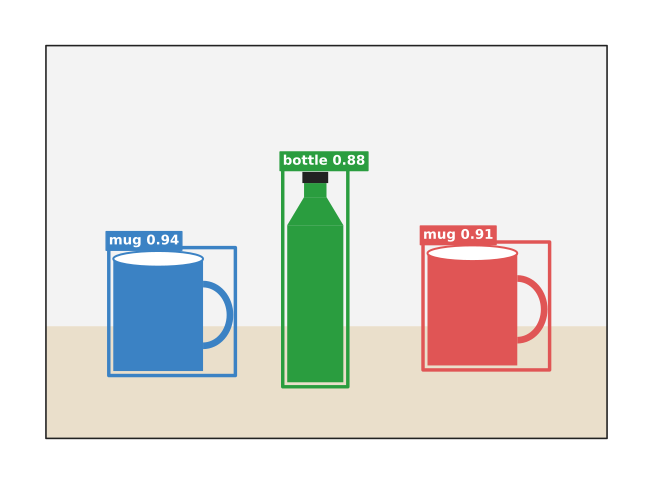
Each box has a tag with the class and the confidence, and those confidence numbers are examples rather than real output.
The list can be empty, which means the model found nothing it knows, and it can also hold objects the model is not at all sure about. So every program that uses a detector sets a confidence threshold, and throws away every box whose confidence is lower than that number. A threshold of 0.25 to 0.5 is a common start. Book 2 discusses this choice in confidence, and the threshold.
3. How it works inside#
That list of boxes has to come from somewhere, and a detector begins the work just as a classifier does. So a backbone turns the picture into grids of numbers that describe edges, parts and objects, and then a detection head turns those grids into boxes. There are three main ways to build that head, and this section takes them in turn. The shortlist in section 5 holds models of all three ways, and each way below names the ones that belong to it.
Two stages: first guess the places, then check each one#
The oldest way of building the head splits the work into two separate steps.
- The first step looks over the backbone's grids and suggests a few hundred places that might hold an object, where each suggestion is a rough box. These suggestions are called region proposals.
- The second step then looks at each proposal on its own, and gives that proposal a class and a confidence, as a classifier would. It also moves the edges of the box a little, so that the box fits the object better.
This way is accurate, but it is slower, because the second step runs once for each proposal. The best-known model of this kind is Faster R-CNN, and section 5.5 recommends it for fine-tuning in plain PyTorch. Faster R-CNN is also the only two-stage model in that shortlist, because the two ways below are both faster.
One stage: look once, answer for every cell#
A faster way does all of that in one step. So the name of the best-known model of this kind says it directly: YOLO, short for "you only look once".
- The picture is split into a grid of cells. A real model uses several grids at once, with small cells for small objects and large cells for large ones.
- For each cell, the head asks: is the middle of an object inside this cell?
- If the answer is yes, that cell gives the object's box, its class and a confidence.
The picture below shows the idea with one coarse grid.
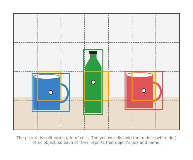
The white dot marks the middle of each object, and the yellow cell around each dot is the cell that reports that object. Its box can be larger than the cell itself, because the backbone's numbers for each cell already carry information about the area around it.
The whole picture goes through the network only once, which is why one-stage detectors are fast enough to run on every frame of a live camera. The one-stage model in the shortlist is Ultralytics YOLO26, the current release of that same YOLO family, and section 5.1 recommends it.
Cleaning up the extra boxes#
Both of the ways described so far share one side effect, because a one-stage or two-stage detector usually gives several boxes for the same object. Nearby cells, or nearby proposals, all see the same mug, and each one of them reports it separately.
So the detector runs a cleanup step after the network, and that step is called non-maximum suppression, or NMS, which works like this.
- Sort all the boxes of one class by confidence, highest first.
- Keep the box with the highest confidence.
- Remove every other box that overlaps the kept box by more than a set amount.
- Repeat with the next highest box that is still left.
The overlap is measured as the area the two boxes share, divided by the area they cover together, and this number is called intersection over union (IoU). It is 1 when the two boxes are the same and 0 when they do not touch at all, so a common setting removes boxes with an IoU above 0.5 or so.
The picture below shows five boxes for one mug, and the one box that is left after the cleanup.
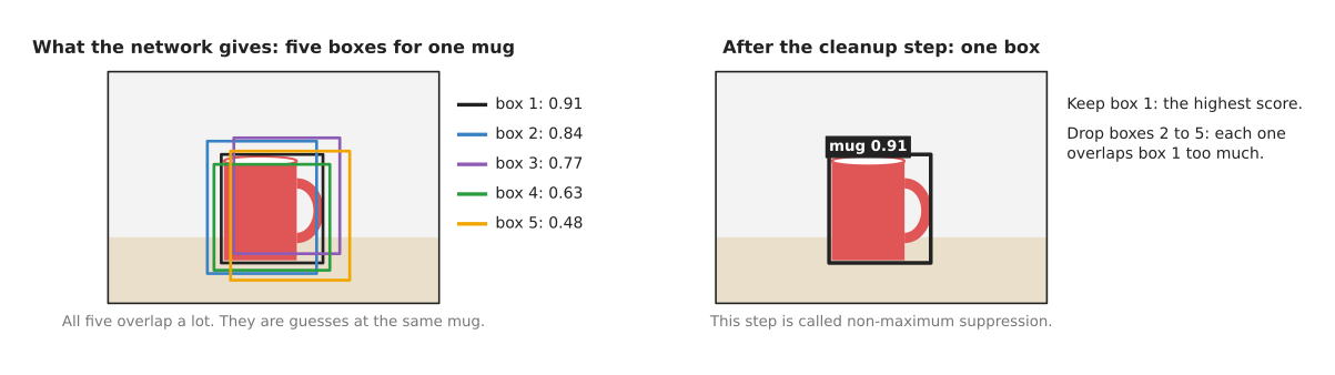
The cleanup has one weakness, because two real objects that stand very close together have boxes that overlap a lot, so the cleanup may then remove one of those boxes by mistake.
Transformers: a fixed set of answers#
A newer way avoids that cleanup step altogether by using a transformer, the kind of network that the classification page mentioned. The first model of this kind was DETR, short for "detection transformer", and it is the clearest one to explain the idea with. The shortlist keeps DETR in section 5.6 for that reason rather than for use on a robot.
- The model starts with a fixed number of empty answer slots, for example 100. These slots are called queries.
- Each query looks at all of the backbone's grids through the attention step, and gathers from them whatever it needs to describe one object.
- Each query then gives one box and one class, and a query that found nothing can give the class "no object" instead.
During training, each real object is matched to exactly one query, so the model learns to give one box per object and needs no cleanup step at all. This is also simpler for the program after the network, and it avoids the weakness with close objects described above.
Three of the models the shortlist recommends for real work are built this way, each changing a different part of DETR's design: RT-DETR in section 5.2, RF-DETR in section 5.3 and D-FINE in section 5.4.
4. How it is trained#
Whichever of those three heads a detector uses, it learns in the same way, from pictures where a person has drawn a box around every object and written its class. This work is called labelling, or annotation, and drawing boxes is quick compared with tracing outlines, but it is still slower than writing one name per picture.
The most used collection is COCO, short for "Common Objects in Context", which has about 120,000 labelled photos for training, with 80 classes. Those classes include "cup", "bottle", "bowl", "scissors" and "person", and most detectors you can download were trained on COCO.
Training a detector works in the same way as training a classifier. The network makes its guesses for a batch of pictures. Then a program compares each guess with the drawn boxes and measures three kinds of error: the box is in the wrong place, the class is wrong, or an object was missed. It then nudges the network's numbers to reduce those errors, and repeats.
A robot project almost always fine-tunes rather than training from nothing. So it starts from a detector trained on COCO and trains it further on its own pictures with its own classes. A few hundred labelled pictures is a common starting point, and Book 2 walks through a complete example with 80 pictures in training a model of your own.
Some projects make their training pictures in a simulator instead. This is because the simulator draws the objects itself and already knows exactly where every box is, so nobody has to label anything by hand. The page where the data comes from explains this.
5. Well-known models#
This section is the shortlist a real project chooses from. For each model it says what the model is, how it works differently from its neighbours, why you would pick it rather than the obvious alternative, what it costs you, and what to type to run it. The cost is one short line near the top of each sub-section, written in the three scales that the chapter overview defines in how this chapter writes size, machine and licence.
Read the table as a shortlist and not as a ranking. The left column names the model and says how current it is. The right column holds everything else about it: the job it is best at, its size, its licence, and when to pick it. A size is given as the number of parameters, which is the count of numbers the network learned during training, written in millions. Every number was read from the project's own published table or model card, and each sub-section names which. Two projects measure on different machines, so treat the sizes as a rough guide to scale.
| Model | What decides it |
|---|---|
| Ultralytics YOLO26, most used in 2026 | It is a one-stage detector, and its five sizes hold 2.4 to 55.7 million parameters under AGPL-3.0 or under a paid Enterprise licence. It is best at getting a working detector running in an afternoon. Pick it when you can publish your own source code, or when you pay for the other licence. |
| RT-DETR, most used in 2026 | It is a transformer detector, and its ResNet-50 checkpoint holds 43.0 million parameters, with Apache-2.0 on both the code and the weights. It is the most familiar permissive transformer detector, because it sits inside a library you may already use. Pick it when you want no licence restriction, and no cleanup step after the network. |
| RF-DETR, worth betting on | It is a transformer detector, and its sizes hold 30.5 to 33.9 million parameters for Nano to Large, and 126.4 and 126.9 million for XL and 2XL. Nano to Large are Apache-2.0, while XL and 2XL are PML 1.0. It gives the best boxes available at a given speed under a permissive licence. Pick it when the licence must stay permissive and the boxes must be good. |
| D-FINE, worth betting on | It is a transformer detector, and its largest checkpoint holds 62.9 million parameters under Apache-2.0. It is best at placing the edges of the box precisely. Pick it when you fine-tune on your own objects and you measure from the box. |
| Faster R-CNN, historical | It is a two-stage detector, and fasterrcnn_resnet50_fpn_v2 holds 43.7 million parameters under BSD-3-Clause. It is best at fine-tuning in plain PyTorch with no new dependency. Pick it when you already use torchvision, and you do not need 30 frames a second. |
| DETR, historical | It is the first transformer detector, and its ResNet-50 checkpoint holds 41.6 million parameters, with Apache-2.0 on both the code and the weights. It is best at explaining how a query-based detector works. Pick it when you are learning the design rather than shipping a robot. |
5.1 Ultralytics YOLO26#
Most used in 2026, because a developer who has never trained a model can install one package and have boxes on their own photo within minutes.
Size xs to s, a laptop for the smallest of its five sizes and a small card for the largest, AGPL-3.0 or a paid Enterprise licence on both the code and the weights.
Ultralytics is the company that publishes the YOLO family as a Python package, and
YOLO26 is its current release. Its
documentation page describes it as
released in January 2026 and cites the paper "Ultralytics YOLO26: Unified Real-Time
End-to-End Vision Models" (arXiv:2606.03748).
The letter in the file name is the size, so yolo26n.pt is the smallest of the five
and yolo26x.pt is the largest.
The one idea YOLO26 is built on is that everything a detector does after the network
should be optional. It is still the one-stage design of section
3, so it still answers for every cell of several grids in a
single pass. What is new is that its documentation describes two heads trained side
by side on one backbone, and you choose which of them answers. The first head is the
familiar one, where many cells report the same object and the cleanup step of section
3 picks one of them. The second head is trained so that only one prediction survives
per object, so there is nothing left to clean up, and you select it by passing
nms=False.
Those two heads give answers of different shapes. The first head produces one row for every cell of every grid, which is several thousand rows for an ordinary picture, and the suppression step then throws nearly all of them away. The second head produces at most 300 rows, and each row is already meant to be a separate object. YOLO26 also changed how the model describes a box edge. Older YOLO heads described each edge as a spread of weights over a row of candidate positions and then took the weighted average, a step named Distribution Focal Loss, and YOLO26 removes it and predicts the distance to each edge as one plain number instead. That makes the head smaller and the export to other formats simpler. It is also the exact opposite of the choice D-FINE makes in section 5.4, which keeps that spread of weights and sharpens it step by step, so the two models disagree about whether an edge is better described by one number or by many.
What the two heads buy you is a choice rather than a compromise, because both are trained whichever one you then use. The second head removes a step whose cost grows with the number of boxes, so a crowded tray no longer slows the program down more than an empty one, and it removes the suppression code from whatever runs on the robot. What it costs is a little accuracy, because the documentation's own table gives the second head a lower score than the first at every size, which is why prediction still uses the first head unless you ask for the other. Describing an edge with one number instead of a spread also gives up some of the precision that the spread bought.
The difference shows up on a robot arm when two copies of the same part lie against
each other in a bin. With the first head their boxes overlap so much that the cleanup
step deletes one of them, so the arm sees one part where there are two, picks it, and
only discovers the second on the next picture. With nms=False both parts keep their
boxes, and the arm can plan two picks from one picture. That is a different answer
from the same file of weights, decided by one argument.
The obvious alternative is RT-DETR in section 5.2, which has a permissive licence. Pick Ultralytics when you are short of time, because it downloads its own weights, it trains on your own pictures with a single call, and almost every tutorial you will find online uses it. Pick RT-DETR instead when your product cannot carry the AGPL-3.0 licence, which obliges you to publish the source of anything you combine Ultralytics with, including software you never hand out but only run as a service for other people. The weights carry the same terms. A paid Enterprise licence removes that obligation and is priced by negotiation, and Book 2 explains the trap in licences, and the one that will catch you out. What goes wrong most often after the licence is the class list, because people assume the 80 COCO classes include their own parts.
The library is ultralytics, which you install with pip install ultralytics.
from ultralytics import YOLO

model = YOLO("yolo26n.pt")                 # the weights download on first use
result = model("table.jpg", conf=0.25)[0]  # conf is the confidence threshold

for box in result.boxes:
    name = result.names[int(box.cls)]
    # xywh is the box as its middle and its size; xyxy would be its two corners.
    middle_u, middle_v, width, height = box.xywh[0].tolist()
    print(f"{name} {float(box.conf):.2f} at pixel ({middle_u:.0f}, {middle_v:.0f})")
You supply the picture and the threshold. The library downloads the weights, resizes
the picture, runs the network, and runs the non-maximum suppression of section
3 for you, or skips it when you pass nms=False. What you
still have to write is everything after the box.
5.2 RT-DETR#
Most used in 2026 among teams that read the licence first, because it is a permissive detector with an API that anyone who has used Hugging Face already knows.
Size s, a small card, Apache-2.0 for the code and the weights.
RT-DETR is short for "real-time detection transformer". Its paper, "DETRs Beat YOLOs on Real-time Object Detection" (arXiv:2304.08069), appeared in April 2023, and it is the model that made the transformer design of section 3 fast enough for a live camera. The weights are published as PekingU/rtdetr_r50vd.
The one idea RT-DETR is built on is that a transformer detector was never slow because of its queries, but because of the attention step that runs over the picture before the queries do. The paper sets out the problem in those terms: YOLO detectors pay for the cleanup step, transformer detectors have no cleanup step but cost too much to compute, so the way forward is to make the expensive part cheap and keep the queries. Everything in the model follows from that one decision.
Inside, the difference from Ultralytics YOLO26 in section 5.1 is not a switch but the whole shape of the answer. YOLO26 must choose between a head that reports from every cell and then suppresses, and a head trained to report once; RT-DETR has no such choice, because the queries of section 3 give one box per object by construction. What RT-DETR changed from DETR is where the attention runs. The paper calls its encoder a hybrid encoder, and the hybrid is that attention between positions runs only inside the smallest of the backbone's grids, the one with the fewest cells and the most meaning in each cell, while the larger grids are joined to it by ordinary convolution-style mixing instead of by attention. The paper describes this as decoupling interaction within one scale from fusion across scales. It then changed where the queries start. In DETR the queries begin as learned vectors that know nothing about the picture in front of them, whereas RT-DETR scores the encoder's own outputs and hands the most promising of them to the decoder as the queries' first guesses, which the paper calls uncertainty-minimal query selection.
What that buys is a detector with no cleanup step at all, and the paper adds a second gain that is unusual: because every decoder layer already produces a complete answer, you can run fewer of them and get a faster, slightly worse detector out of the same file of weights, with no retraining. What it costs is rigidity in the input and in the output. The library's own page states the model expects 640 by 640 and that other sizes usually make it worse, so you cannot trade picture size for speed the way you can with a YOLO model. The number of answer slots is fixed as well, so a picture with more objects than slots loses some of them. Fine-tuning means writing a training loop rather than calling one method.
The difference shows up on a robot arm with two cups standing against each other. With YOLO26's default head one of those two boxes is deleted by the suppression step, and with RT-DETR there is no suppression step to delete it, so both cups are reported every time rather than only when they happen to stand apart. The decoder-layer gain shows up in a second place: one checkpoint can run shallow and fast while the arm is moving and deep and careful for the single picture taken before the grasp, where matching that with a YOLO model would mean shipping two different sizes of weights.
The obvious alternative is Ultralytics YOLO26. Pick RT-DETR when you are building something you will sell or run as a service without publishing its source, because both the code and the weights are Apache-2.0, which puts no such condition on you. Pick Ultralytics when the input size has to vary, or when you want a one-line training call.
The library is transformers, which you install with pip install transformers.
The code below is the example from the library's
RT-DETR page,
shortened.
import torch
from PIL import Image
from transformers import RTDetrForObjectDetection, RTDetrImageProcessor

processor = RTDetrImageProcessor.from_pretrained("PekingU/rtdetr_r50vd")
model = RTDetrForObjectDetection.from_pretrained("PekingU/rtdetr_r50vd")

image = Image.open("table.jpg")
inputs = processor(images=image, return_tensors="pt")
with torch.no_grad():
    outputs = model(**inputs)

# target_sizes wants the height first, so that the boxes come back in the
# original picture's pixels rather than in the resized picture's pixels.
results = processor.post_process_object_detection(
    outputs, target_sizes=torch.tensor([(image.height, image.width)]), threshold=0.3
)[0]
for score, label, box in zip(results["scores"], results["labels"], results["boxes"]):
    print(model.config.id2label[label.item()], round(score.item(), 2), box.tolist())
You supply the picture and the threshold, as before. The processor resizes the
picture and scales the boxes back to it, and the model carries the 80 COCO class
names, which is why id2label can give you the word "cup". What you have to supply
yourself is a graphics card if you want this on every frame of a live camera.
5.3 RF-DETR#
Worth betting on, because it is the direction the field is going: a transformer detector with a permissive licence that beats the YOLO family on accuracy at the same latency, measured by its authors in one harness rather than quoted from separate papers.
Size s for Nano to Large and m for XL and 2XL, a small card, Apache-2.0 for Nano to Large and a licence called PML 1.0 for XL and 2XL.
RF-DETR comes from Roboflow, a company that sells computer vision tooling, with co-authors at Carnegie Mellon University. Its paper "RF-DETR: Neural Architecture Search for Real-Time Detection Transformers" (arXiv:2511.09554) is from November 2025, and its repository publishes six sizes, from Nano to 2XLarge.
The one idea RF-DETR is built on is that the shape of the network should be measured rather than chosen. The paper's method is neural architecture search, usually shortened to NAS, which means letting a program try very many network shapes and keep the ones that measure best. Every other model in this section is a shape somebody designed and then trained. RF-DETR's six published sizes are shapes a search found.
Two things differ from RT-DETR in section 5.2, which is the transformer detector just above. The first is the backbone. RT-DETR's backbone is a ResNet trained to put a name on a whole picture, whereas RF-DETR's backbone is DINOv2, a vision transformer trained on a large collection of pictures with no labels at all, which the paper credits for carrying over to objects that its training never named. The second is the search itself. The authors train one network whose parts share their weights, so that its width, its depth and the size of picture it takes can all be varied after training without any part being retrained. They then measure thousands of those settings on the dataset they care about and keep the ones that sit on the best accuracy-against-latency curve. The repository says the same search now runs on the company's platform for your own dataset. The queries, the decoder and the absence of a cleanup step are inherited rather than invented, and the repository credits LW-DETR, DINOv2 and Deformable DETR as the work it is built on.
What the search buys is that you choose a point on a curve that was measured, instead of hoping that a hand-designed size happens to land where your robot needs it. The unlabelled pre-training buys the other half: the paper's headline comparison is not only on COCO but on RF100-VL, a collection of real-world datasets whose classes were not in any of these models' pre-training. What it costs is that the model cannot be made very small, because a DINOv2 backbone is not a tiny network, so there is no very small RF-DETR for a very small computer. The search for your own data belongs to the company's platform rather than to the package, and the package is young enough that its API still changes between releases.
The difference shows up on a robot arm when your parts look nothing like anything in COCO, for example dark brushed-metal fittings on a dark tray. That is the case RF100-VL is built to measure, so the gap the paper reports there is the gap you are likely to see, and it changes how many of your own pictures you have to label before the boxes are good enough to pick from. On a tray of cups and bottles the two models are much closer, and the choice goes back to the licence and the tooling.
The obvious alternative is again Ultralytics YOLO26, because the two packages are
about equally easy to use. Pick RF-DETR when you want the permissive licence and the
better boxes at once. Its README reports every row measured in one harness on the
5,000 pictures of the COCO validation split, with latency on an NVIDIA T4 graphics
card using TensorRT: RF-DETR-Nano reaches 48.4 average precision at 2.3
milliseconds, where YOLO26-N reaches 40.3 at 1.7 milliseconds. Those are the
authors' measurements of their own model against a competitor, so read them as a
claim with a method attached rather than as a neutral result. The licence split is
the thing to check before you commit: the README states that XL and 2XL live in a
separate rfdetr_plus package under PML 1.0, so the permissive promise covers Nano,
Small, Medium and Large only.
The library is rfdetr, which you install with pip install rfdetr. It returns
its answers as a Detections object from the supervision library, which is the
same type several other detectors in this family use.
from rfdetr import RFDETRMedium
from rfdetr.assets.coco_classes import COCO_CLASSES

model = RFDETRMedium()                    # replace with RFDETRNano for the small one
detections = model.predict("table.jpg", threshold=0.5)

for class_id, confidence, box in zip(detections.class_id, detections.confidence,
                                     detections.xyxy):
    # xyxy is the box as its left, top, right and bottom edges, in pixels.
    print(COCO_CLASSES[class_id], round(float(confidence), 2), box.tolist())
You supply the picture and the threshold, and the package downloads the weights and
returns boxes in your picture's pixels. The COCO_CLASSES list above applies only to
the COCO-trained weights, and the README says to read detections.data["class_name"]
instead once you have fine-tuned the model on your own classes.
5.4 D-FINE#
Worth betting on for work where the edges of the box have to be right, because it changes how the network predicts those edges rather than how fast it runs.
Size s, a small card, Apache-2.0 for the code and the weights.
D-FINE is a detection transformer from the paper "D-FINE: Redefine Regression Task in DETRs as Fine-grained Distribution Refinement" (arXiv:2410.13842), its code is at Peterande/D-FINE, and its largest weights are published as ustc-community/dfine_x_coco. The Hugging Face D-FINE page summarises the paper's results as 54.0 and 55.8 average precision on COCO for the Large and XLarge sizes, at 124 and 78 frames a second on an NVIDIA T4 graphics card.
The one idea D-FINE is built on is that the position of a box edge should be given as a set of possibilities rather than as a single number. Every other detector in this section finishes by printing four numbers for a box. D-FINE instead keeps, for each of the four edges, a row of candidate positions near the current guess together with a weight for each candidate, meaning "the edge is most likely here, a little less likely one step to the left, a little less one step to the right". The paper calls this fine-grained distribution refinement, and refinement is the second half of the idea: each layer of the decoder sharpens that row of weights instead of starting a new guess from nothing.
Everything else is RT-DETR from section 5.2, which D-FINE is built from, so the queries, the decoder and the absence of a cleanup step are unchanged. Two things in the last part of the model are not. The first is the one just described: where RT-DETR's layers each predict a correction to four numbers and the last layer's answer is the one used, D-FINE's layers each update the weights over candidate positions and the final edge is the weighted average of them. The second is how the layers teach each other. The paper's second component is self-distillation, which means that the model's own later output is used as the training target for its earlier output: the sharp set of weights the deepest layer arrives at becomes what the shallow layers are trained to aim for, so a shallow layer has a precise target instead of a vague one. It is worth putting this next to Ultralytics YOLO26 in section 5.1, because YOLO26 deleted exactly this kind of spread of weights from its own head to make it smaller and simpler to export. The two projects made opposite decisions about the same part of a detector, and each decision follows from what the project cares about: YOLO26 wants a cheap head, D-FINE wants an exact edge.
What the idea buys is localisation, which is the word for how close a predicted edge is to the real one, and the paper reports that bolting these two components onto other detection transformers raised their accuracy for almost no extra parameters. What it costs is understanding and company. The last part of the model is harder to follow and harder to debug than four numbers, and the model is far less written about than RT-DETR, so fewer people have published training settings that work. If your program only ever uses the middle of the box, the idea buys you nothing at all.
The difference shows up on a robot arm when you read something off the box other than its middle. Two examples: measuring an object's width in pixels to tell a 40 millimetre fitting from a 45 millimetre one, and cutting the box out of the picture to hand to a segmentation model. In both cases an edge that is three pixels out changes the answer, and in the second case a box that is slightly too tight cuts a piece off the object before the next model ever sees it. If you are only pointing the gripper at the middle of the box, pick RT-DETR and spend the attention somewhere else.
The obvious alternative is RT-DETR, which D-FINE is built from. Pick D-FINE when you do something with the box edges other than point at the middle, because that is the part it improves. Pick RT-DETR when you want the older and more widely used model, which has more tutorials and more people who have met your problem already.
The library is transformers again, and the code differs from section 5.2 in two
lines only, which is the practical reason to prefer Hugging Face over each
project's own repository.
from transformers import AutoImageProcessor, DFineForObjectDetection

processor = AutoImageProcessor.from_pretrained("ustc-community/dfine_x_coco")
model = DFineForObjectDetection.from_pretrained("ustc-community/dfine_x_coco")
# Everything after this point is the RT-DETR code of section 5.2, unchanged,
# because post_process_object_detection is shared by both models.
What you supply is the same as for RT-DETR. What the library gives you is one interface over many detectors, so swapping the two names above compares two models on your own photos in an afternoon.
5.5 Faster R-CNN#
Historical, kept because it is the two-stage design of section 3 in a library you already have, and because it is still the shortest way to fine-tune a detector without adding a dependency.
Size s, a small card, BSD-3-Clause for the code and the weights together, which is the most permissive licence in this section.
Faster R-CNN was published in 2015, and its name comes from "region-based
convolutional neural network". It established the two-step shape: suggest a few
hundred places, then classify each one. It ships inside torchvision, the image half
of PyTorch, and the newer of its two versions is fasterrcnn_resnet50_fpn_v2.
The one idea Faster R-CNN is built on is that the places worth looking at should be suggested by the same network that then classifies them. The two-stage detectors before it got their region proposals from a separate hand-written program, and the paper says plainly that this program had become the slow part. So Faster R-CNN adds a small network, the region proposal network, that reads the backbone's grids directly. Because it shares those grids with the classifying step, the proposals cost almost nothing extra, and the paper describes the proposal network as telling the rest of the model where to look.
Inside, that proposal network slides over the shared grid and, at every position, considers a small fixed set of candidate rectangles of different shapes and sizes. Those candidates are called anchors. For each anchor it answers two questions: does this rectangle contain an object at all, and how should its edges move to fit the object better. The few hundred best-scoring anchors become the proposals, and the second step then cuts each proposal's patch out of the shared grid, resizes that patch to a fixed small square, and classifies it. This is where it differs from every model above it: the class decision is made separately for each cut-out patch, rather than for a grid cell as in Ultralytics YOLO26, or by a query that looked at the whole picture as in RT-DETR, RF-DETR and D-FINE. A proposal sees only its own patch, so two proposals that both found the same mug cannot know about each other, and that is exactly why the suppression step of section 3 is unavoidable here rather than optional.
What the design buys is a careful second look at each candidate, and a training path short enough to read end to end, which is why it survives as the model people fine-tune when they want to understand every line. What it costs is time that depends on the picture. The second step runs once per proposal, so a tray holding thirty objects takes longer than an empty table, where a one-stage detector costs the same either way. It is the slowest model in this section, and it still needs the cleanup step together with its weakness for objects that touch.
The difference shows up on a robot arm as a surprise about speed rather than about accuracy. A team measures Faster R-CNN on a test photo of one mug, sees a frame rate they can live with, and then puts a full tray in front of the camera and finds the loop much slower, because the amount of work grew with the number of objects. A one-stage detector measured on the same two pictures gives almost the same time for both. So Faster R-CNN is the right choice when the camera takes one careful picture and the program has a second to think, and the wrong one when the number of objects in view is unpredictable.
The obvious alternative is any of the four models above, all of which are faster. Pick Faster R-CNN anyway when your project is already a PyTorch project, when you want to fine-tune with code you can read end to end, and when the camera gives you a picture every second rather than thirty times a second. The torchvision model page gives this version 46.7 box mAP on the COCO validation split and states no speed at all, so measure it on your own pictures before you promise anyone a frame rate.
The library is torchvision, which arrives with PyTorch.
import torch
from torchvision.io import decode_image
from torchvision.models.detection import (fasterrcnn_resnet50_fpn_v2,
                                          FasterRCNN_ResNet50_FPN_V2_Weights)

weights = FasterRCNN_ResNet50_FPN_V2_Weights.DEFAULT
model = fasterrcnn_resnet50_fpn_v2(weights=weights).eval()

image = decode_image("table.jpg")
# weights.transforms() is the exact preparation these weights were trained with.
batch = [weights.transforms()(image)]
with torch.no_grad():
    prediction = model(batch)[0]

for label, score, box in zip(prediction["labels"], prediction["scores"],
                             prediction["boxes"]):
    if score > 0.5:                       # torchvision applies no threshold for you
        print(weights.meta["categories"][label], round(float(score), 2), box.tolist())
You supply the picture and, this time, the threshold test itself, because torchvision
returns every box the network produced. The weights.transforms() call is the part
worth copying, because getting that preparation wrong is the usual reason a
torchvision model gives poor answers.
5.6 DETR#
Historical, kept because it explains the query idea that RT-DETR, RF-DETR and D-FINE are all built on.
Size s, a small card, Apache-2.0 for the code and the weights.
DETR, short for "detection transformer", came from Facebook AI Research in 2020, and it is the model section 3 describes under "a fixed set of answers". Each of its 100 queries gives one box or the answer "no object", and the paper's title for what it does is direct set prediction.
The one idea DETR is built on is that a detector should output a set, and should be trained as if it output a set. Training is where that idea lives. For each picture, a program pairs up the model's predictions with the real objects, one prediction to one object, choosing whichever pairing costs least over the whole picture. The paper calls this bipartite matching, and bipartite matching means nothing more than matching the members of two lists one to one, with no member used twice. Every prediction left unpaired is trained to say "no object". That single rule is what removes the cleanup step, because a prediction is rewarded only when it is the one chosen for an object, so producing a second box for an object that another prediction already took is punished rather than tolerated.
Inside, that means DETR throws away almost everything Faster R-CNN in section 5.5 uses. There are no anchors, no region proposals, and no suppression. The backbone's grid goes through a transformer encoder, and a fixed set of learned query vectors goes through a decoder in which each query attends both to the whole encoded picture and to the other queries. That second part is the piece worth holding on to: the queries can take each other into account, which is how they divide the objects between themselves without being told to. Faster R-CNN's anchors and YOLO's grid cells have no way to do this, because each one is scored on its own, and that is why those designs need a step afterwards to decide who wins.
What the idea buys is simplicity and reach, and the paper shows it extending to panoptic segmentation, where every pixel is labelled, without a new design. What it cost DETR itself was training time and small objects. Its published training schedule is far longer than a one-stage detector's of the same year, and it was poor at finding small objects, because its attention ran over a single coarse grid with no fine grid to place a small thing on. Each of the three models above repairs one of those faults: RT-DETR gives the encoder several scales cheaply and starts the queries from the picture rather than from nothing, D-FINE replaces the four numbers with sharpened distributions, and RF-DETR searches for the shape instead of designing it.
The difference does not show up on a robot arm, because there is no case for putting DETR on one. Where it shows up is on your screen: run the code below, print all 100 answers without a threshold, and watch most of them say "no object". Reading that list once makes the three recommended transformer detectors above understandable in a way no description does, because you can see that the model produced a fixed-size set and filled only as much of it as the picture needed.
The obvious alternative is RT-DETR, which is the same idea made fast. Pick DETR only to read, and its weakness is the reason the later models exist. Its licence is Apache-2.0 for both code and weights, read from the model card.
The library is transformers, and the code is the RT-DETR code of section 5.2 with
the names changed.
from transformers import AutoImageProcessor, AutoModelForObjectDetection

processor = AutoImageProcessor.from_pretrained("facebook/detr-resnet-50")
model = AutoModelForObjectDetection.from_pretrained("facebook/detr-resnet-50")
# The rest is section 5.2's code, because the post-processing call is the same.
What you supply is a picture. What you get back is a list of 100 answers of which most say "no object", and that is the clearest way to see what a query-based detector does.
5.7 How to choose#
Start with Ultralytics YOLO26 if you may publish your source code or pay for the Enterprise licence, because nothing else gets you from an empty folder to boxes on your own photo as quickly.
Four things change that answer.
- You are selling a product, or running a service, and will not publish your source. Then the AGPL licence rules Ultralytics out, and you take RF-DETR for the best boxes or RT-DETR for the most familiar code. Check that you stay within RF-DETR's Nano to Large sizes, because XL and 2XL are under a different licence.
- The computer has no graphics card. Then take the smallest Ultralytics checkpoint, measure it on your own pictures, and read running a model on a robot before you promise anyone a frame rate.
- Your objects stand against each other, or they overlap. Then prefer a model
that needs no cleanup step, which means RT-DETR, RF-DETR, D-FINE, or Ultralytics
with
nms=False, because the suppression step is what loses one of two touching objects. - Your objects are not among the 80 COCO classes. Then the model matters less than the labelling, because you will fine-tune whichever one you pick. Choose the one whose training code you can live with, which today usually means Ultralytics or RF-DETR.
If you cannot list your objects in advance at all, no model in this section will find them, and the page you want is open-vocabulary models. Book 2's models that find objects lists more detectors, each with the licence read from its own licence file.
6. Where this is going#
The sections above describe detectors that exist now, and this one is about what happens next. It follows the rule set out in four kinds of claim, and why the difference decides everything: a demonstration shows something working once, a product announcement says a thing can be bought or downloaded and is therefore checkable, a research result is a measured number with a stated method, and a projection names a date that has not arrived. Every paragraph below says which of those it rests on, and says when a judgement is mine.
How it got here#
Detection has moved in one direction for ten years, and the direction is that each hand-written step has been deleted. Faster R-CNN in section 5.5 replaced a hand-written region proposer with a network that proposes regions. YOLO deleted the second pass over each proposal. DETR deleted the anchors and the cleanup step. Ultralytics YOLO26 in section 5.1 makes that cleanup step optional inside the one-stage design too. The step being deleted now is the class list itself, and the models that delete it are on the page open-vocabulary models.
Where it is used in industry today#
Detection is in production in warehouses, and the clearest published case is Amazon's. Amazon's own page for Sparrow, the arm that moves individual products between totes before they are packed, says Sparrow uses computer vision and artificial intelligence and "can recognize and handle millions of items". That is a product announcement about a system Amazon runs in its own buildings, not about something you can buy. What you can buy is the perception layer that integrators put on their own arms. Plus One Robotics sells PickOne, whose product page says it analyses two-dimensional, three-dimensional and model output together to decide the robot's commands at a depalletising station where the boxes vary and overhang the pallet. RightHand Robotics lists RightPick AI as the perception part of its piece-picking system. Ambi Robotics sells AmbiSort for putting parcels into sort bins and AmbiVision for reading them, and the AmbiVision page describes a station that photographs a box from every side and runs those pictures through a model to find the identifiers it was asked for, computing on site rather than in a data centre.
Inspection on a production line is the second large use, and there a detector is usually sold inside a machine vision library rather than downloaded. MVTec sells HALCON and MERLIC, and its deep learning methods page recommends its object detection for pick-and-place, assembly inspection and robot vision. Its named deployments are the part worth reading. MVTec's own case study says Panasonic Energy uses HALCON's deep learning at its Kansas plant to inspect cylindrical lithium-ion batteries after slitting, including the laser weld marks on the electrode tabs, and reports a 57.3 per cent reduction in over-detections in the trial that preceded it, which is the vendor's own figure from the vendor's own trial. Cognex sells the same kind of tool and is the best-known company in this market, but its website refuses an automated request, so this page names it without a link. Smaller companies sell the whole station rather than the library: Instrumental inspects electronics assembly and names Meta and NVIDIA as customers on its own home page, and Elementary sells camera stations for defect detection, label verification and presence checks.
Agriculture is where a detector runs on the largest number of machines, because one sprayer covers a field. John Deere sells See & Spray, and Blue River Technology, the Deere subsidiary that builds it, says on its own site that See & Spray "uses computer vision and machine learning to distinguish crops from weeds". Carbon Robotics sells the LaserWeeder, which kills weeds with lasers rather than herbicide, and its specification page is unusually detailed for a vendor page: 42 high-resolution cameras, 30 diode lasers of 150 watts each, more than 100 deep-learning crop models, and more than 100 growers across North America, Europe and Australia operating the implement since February 2022. Those are the company's own figures and nobody independent has published a check of them. What makes agriculture the strongest case on this page is the job itself, because the machine has to decide plant by plant at tractor speed.
What is being worked on right now#
The first front is the one section 5 already shows: the transformer detector is being made cheaper to train and faster to run, one component at a time. D-FINE changed how a box edge is predicted. DEIM, from the paper "DEIM: DETR with Improved Matching for Fast Convergence" (arXiv:2412.04234), changed how predictions are matched to real objects during training so that fewer passes over the data are needed, and its code is Apache-2.0. RF-DETR stopped designing the shape of the network and searched for it instead. These are research results with public code and published numbers, and together they mean a permissively licensed transformer detector is now a default rather than a sacrifice.
The second front is removing the class list. An open-vocabulary detector takes words instead of a trained list, so adding a class costs a sentence instead of a labelling campaign. Grounding DINO and OWLv2 are the permissive ones, YOLOE is the fast one, and open-vocabulary models covers the family with each licence read from its own licence file. The measured form of the claim is RF100-VL, a collection of real-world datasets whose classes are in none of these models' pre-training, which is why RF-DETR's paper uses it for its headline comparison. Half of this is already a product: Roboflow's documentation for AI labelling describes Auto Label, which labels a whole dataset with a foundation model, and Box Prompting, which finds every other instance of a thing in a picture after you draw two or three examples. So what you can buy today removes the labelling, not the trained detector.
The third front is the computer on the robot. The cleanup step of
section 3 is awkward to export, because it is a loop whose
cost depends on how many boxes there are, which is why YOLO26's nms=False head and
the whole DETR family matter more for deployment than for accuracy. The other half is
arithmetic precision, because accelerators such as the
Hailo-8 run a
fixed set of operations on low-precision numbers, so a model must be converted before
it runs there at all. Running a model on a
robot
covers the measurement side.
The fourth front is the measuring stick, and it is the one a reader is least likely to have heard of. COCO's labels are now worse than the detectors measured against them. The paper "Benchmarking Object Detectors with COCO: A New Path Forward" (arXiv:2403.18819) inspected thousands of COCO masks, found imprecise boundaries, missing instances and mislabelled masks, published corrected annotations as COCO-ReM, and reports that of fifty detectors evaluated, those predicting sharper outlines score higher against the corrected labels. The consequence for a robot team is blunt: a few tenths of a point of average precision between two models on COCO is not evidence about your own parts.
What is still unsolved#
A detector reports what it can see, and it cannot report the part of an object that something else covers. The research name for the missing ability is amodal segmentation, which means predicting the whole of an object including its hidden part, and it has been a named problem since "Amodal Instance Segmentation" (arXiv:1604.08202) in 2016. Recent work such as pix2gestalt (arXiv:2401.14398) draws the whole object by generating the missing part. Ten years on, that work is still research results on datasets and I know of no product that sells it. For a robot arm this is the difference between emptying a bin and picking the top item, taking a new picture, and starting again.
Transparent and shiny objects are the second unsolved case, and the record is long enough to be instructive. ClearGrasp (arXiv:1910.02550) appeared in 2019 and TransCG (arXiv:2202.08471) in 2022, and both are datasets with a baseline rather than a method anybody ships. A glass has no reliable edge in a colour picture and no reliable surface in a depth picture, so both signals a detector relies on fail at once. A foundation model with a keeper works through what this does to a real program.
The third unsolved thing is the confidence number. It is not a probability, and it does not fall when the camera is shown something the model has never seen, so a detector trained on 80 classes will happily put 0.8 on a part belonging to none of them. Every project therefore checks the detector with something else, such as a size test or a depth test. I have not found a detector that ships a calibrated confidence, which is a statement about what I could find rather than proof that none exists.
The next two to three years#
I expect permissively licensed transformer detectors to take most new commercial work from the YOLO family, and the reason is the licence rather than the accuracy. This is my expectation and not an announcement by anybody, but the part underneath it is checkable. Ultralytics is AGPL-3.0 on code and weights, which obliges you to publish the source of what you combine it with, including software you only run as a service, and the alternative is an Enterprise licence priced by negotiation. RT-DETR, D-FINE and DEIM are Apache-2.0, and RF-DETR is Apache-2.0 from Nano to Large. Two years ago the permissive option cost you accuracy, and section 5.3 holds the measurements saying it no longer does. A product team's lawyer reads the licence before the benchmark.
I expect open-vocabulary detection to become normal at labelling time and to stay unusual at run time. The labelling half is a product today, which you can check on the Roboflow page linked above. The run-time half has two problems nobody has solved. It is slower, because the model processes the words as well as the picture. And it is not repeatable, because two reasonable wordings of one request return different sets of objects, which is hard to defend where an inspection must give the same answer tomorrow. So the shape I expect is an open-vocabulary model labelling your pictures and a small closed-set detector trained on those labels running on the line. What would disprove it is a vendor shipping an open-vocabulary detector with a stated frame rate and a stated repeatability figure.
I expect the cleanup step to disappear from most deployed detectors, and the reason is deployment rather than accuracy. Both design families have arrived there from opposite directions, which is the strongest evidence a prediction of this kind can have: the DETR family never had the step, and YOLO26 has added a head that does not need it. The step costs more as the picture gets busier, it is the awkward part of an export, and it is what loses one of two objects that touch. None of those reasons depends on anybody's roadmap.
I expect the numbers quoted at robot teams to move off COCO. The reason is the research result above, that COCO's own labels are the limit of what it can measure, so a model can now look better on COCO partly by matching its mistakes. RF100-VL rewards what a robot team cares about instead, which is how a model behaves on objects that were not in its pre-training. This is already visible in how RF-DETR's authors report their own work, and I expect others to follow, because a project reporting only COCO starts to look like it is avoiding the harder measurement.
One more direction is worth naming and worth distrusting. Several groups are folding detection into a larger model that also answers questions, of which ChatRex (arXiv:2411.18363) is one example, so a robot would ask one model for the boxes and the reasoning together. These are research results on benchmarks, the models are far too slow for a live camera, and nothing in this direction is sold. I do not expect it to replace a detector in a robot cell within three years, and I record that here so it can be checked later.
7. Where to read next#
- The next page is segmentation, which replaces the box with the exact outline of each object.
- Image classification explains the backbone and the fine-tuning that every detector uses.
- Open-vocabulary models find objects from a word, without training on them first.
- Tracking and motion follows detected objects from one picture to the next.
- Running a model on a robot explains how fast a model must be, and where it runs.
- Book 2 goes deeper in finding an object in a picture, which runs a real YOLO detector, and in models that find objects.