This page explains the simplest seeing model, which is one that looks at a whole picture and gives it one name. It answers five questions: what such a model does, what goes in and what comes out, how it works inside, how it is trained, and when it is the right choice for a robot arm.
It is written for a reader who has already read the seeing models overview and the first chapter of this book, but you do not need to know any machine learning, because every term is explained where it first appears.
This page comes first in the chapter for a reason, since nearly every other seeing model contains an image classifier, or most of one. So the ideas here come back on every later page.
Contents#
- What it is
- What goes in and what comes out
- How it works inside
- How it is trained
- Well-known models
- Where this is going
- Where to read next
1. What it is#
An image classifier is a model that looks at a picture and says which one of a fixed list of names fits it best.
That fixed list is chosen before training, and each name on the list is called a class. A class can be a kind of object, such as "mug", "bowl" or "bottle", and it can also be a state, such as "gripper empty" or "gripper holding something".
Here is an everyday example: imagine a sorting machine for fruit, where a camera takes a photo of each piece of fruit on a belt. A person could look at each photo and say "apple", "orange" or "lemon". So an image classifier does the same, because it looks at the photo and picks one of the three names.
The classifier gives one name for the whole picture. So it does not say where in the picture the object is, and it does not say how many objects there are either. If a photo shows two apples and an orange, a classifier still gives just one name. The object detection page covers models that find each object separately.
2. What goes in and what comes out#
The input is one picture, and to a computer a picture is simply a grid of numbers. Each small square of the grid is a pixel, and a grey picture has one number per pixel, which says how bright that pixel is. So the number 0 means black, and the number 255 means white. A colour picture has three numbers per pixel instead, one for red, one for green and one for blue.
The picture below shows a tiny grey picture of a mug, and the numbers inside one corner of it.
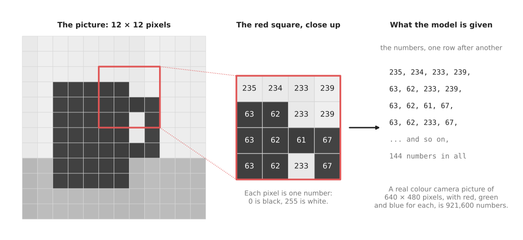
The left part is the picture, 12 pixels wide and 12 pixels high, while the middle part enlarges the red square and writes each pixel's number in it. The right part is what the model is actually given: the same numbers, one row after another.
A real camera picture is much bigger than that. For example, a picture 640 pixels wide and 480 pixels high has 307,200 pixels, and with three colour numbers each, that is 921,600 numbers. So most classifiers first shrink the picture to a fixed size, often a square about 224 pixels wide, so that every picture gives the same count of numbers.
The output is one score for each class, where a score is a number between 0 and 1. So a higher score means the model is more sure that the class fits. The scores for all the classes add up to 1, and the answer is the class with the highest score.
The picture below shows a picture of a mug going in, and five scores coming out.
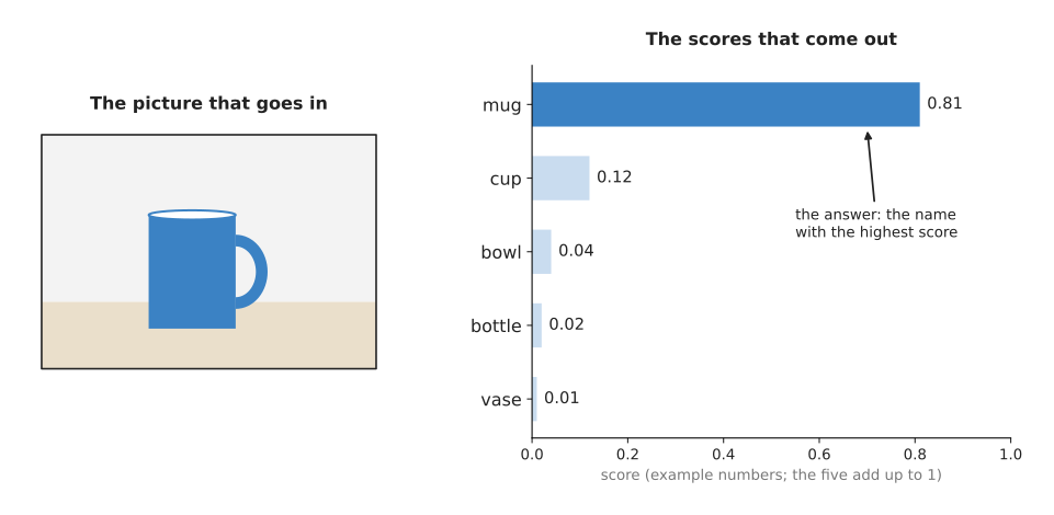
The numbers in this picture are an example rather than real output. In the example, "mug" has the highest score, 0.81, so the answer is "mug", while the second-highest score is for "cup", which is a similar object. This is typical, because a classifier that is wrong is usually wrong in favour of a similar-looking class.
On a robot arm, the input is usually one picture from the camera, or a small part cut out of it. Then the output is used as a yes-or-no check, or to choose what to do next.
3. How it works inside#
A classifier is a neural network, and it is built in layers. This means that each layer takes a grid of numbers in, does simple sums on it, and passes a new grid of numbers on to the next layer. The page inside a neural network explains layers in general, while this section explains what the layers of a classifier do in particular.
The most common kind of classifier is a convolutional neural network (CNN), and a CNN works in these steps.
- The first layer slides a small square, often 3 pixels by 3 pixels, across the whole picture. At each place, it multiplies the 9 pixel numbers by 9 fixed numbers and adds them up, and this sliding sum is called a convolution. The 9 fixed numbers are called a filter, and the layer has many filters, so each one gives its own new grid.
- Some filters give a large number where there is an edge in the picture, so one filter reacts to flat edges, another reacts to upright edges, and another reacts to curves. Nobody chooses these filters by hand, because training finds them.
- Every few layers, the grid is made smaller. For example, each square of 2 by 2 numbers is replaced by the largest of the four, which keeps the important numbers and throws away where exactly they were.
- The next layers do the same thing again, on the smaller grids, and because they combine edges, their filters react to parts: a round rim, a handle loop, or the neck of a bottle.
- The last layers then combine those parts, so their numbers react to whole objects: a mug, a bottle, a bowl.
- At the very end, one small layer turns those numbers into one score per class, and a last step makes the scores positive and makes them add up to 1.
The picture below shows this build-up, from edges to parts to whole objects.
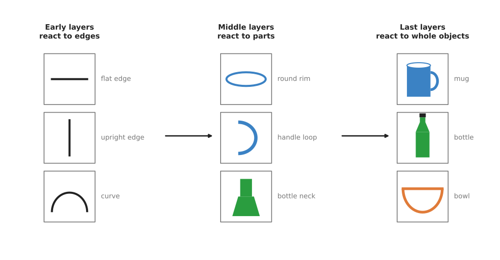
The drawings in the tiles show the kind of pattern that makes each layer give a large number. Researchers have looked inside trained networks, and they found this same order again and again.
Both of the convolutional networks on this page's shortlist are built in those steps: ResNet-50, in section 5.1, and MobileNetV3, in section 5.2. ResNet added one thing to the list above, and the later networks all kept it. In a network of many layers, the output of one layer is also added, unchanged, to the output of a layer two or three further on, and that added shortcut is called a skip connection. It gives the early layers a short path back to the score, so a network of fifty layers trains as well as a short one.
A newer kind of classifier is the vision transformer (ViT), which cuts the picture into small squares, called patches, often 16 pixels by 16 pixels. Then it turns each patch into a list of numbers. After that, each patch's numbers are updated by looking at all the other patches, and this step is called attention. After many such layers the model gives the scores. A vision transformer needs more training pictures than a CNN, but with enough pictures it is often more accurate. The two large backbones on the shortlist are vision transformers: DINOv2, in section 5.3, and DINOv3, in section 5.5.
The part of the network before the last layer is called the backbone, while the last layer, which gives the scores, is called the head. This split matters, because a backbone trained for classification has learned edges, parts and objects, so other seeing models can reuse that backbone and change only the head.
The split also decides how you get a classifier of your own, and section 5 sets out three ways of doing that. The first way trains a backbone and a head together on your own pictures. The second leaves somebody else's backbone exactly as it is and trains only a new head on top of it. The third way has no head with one output per class at all, so it takes a word of explanation here. A vision-language model is two networks: one turns a picture into a list of numbers, and the other turns a sentence into a list of numbers of the same length. The two were trained together on pictures paired with the sentences that describe them, so that a picture and a true description of it come out as nearly the same numbers. You then write each of your class names as a sentence, and a class's score is how close its sentence's numbers are to the picture's numbers. SigLIP 2, in section 5.4, works this way, and nothing in it is trained by you, which is why that third way asks for no pictures of your own.
4. How it is trained#
Training needs many pictures, and each picture needs a label, which is the correct class written down by a person.
The most famous collection of labelled pictures is ImageNet, and the part of it used in a yearly research contest has about 1.2 million training pictures, split into 1,000 classes. Those classes include many animals and everyday objects, such as "coffee mug", "water bottle" and "screwdriver".
Training itself then works in the five steps below.
- The network starts with random numbers in its filters, so its answers are random too.
- It is shown a small batch of pictures, for example 32 of them.
- For each picture it gives its scores, and a program then measures how wrong they are, where the answer counts as very wrong if the correct class got a low score.
- The program nudges every filter number a tiny amount, in the direction that makes the answers less wrong.
- This repeats with the next batch, and so on, many times through all the pictures.
The page how a model learns explains this nudging in more detail.
Training from nothing on ImageNet takes many hours on many graphics cards, so a robot project almost never does that. Instead it starts from a network that someone else already trained on ImageNet, replaces the head with a new one for its own classes, such as "gripper empty" and "gripper holding something", and then trains a little more on its own pictures, which is called fine-tuning.
Fine-tuning works with far fewer pictures, often a few hundred per class, because the backbone already knows edges and parts, and those are the same in every picture. So only the head has much left to learn. Book 2 shows the same idea for a detector in fine-tuning: why 80 pictures are enough.
5. Well-known models#
This section names the models a developer actually reaches for in 2026, and it helps you decide which one to use. It also helps you decide whether you need a classifier of your own at all.
Almost nobody trains a classifier from nothing any more, for the reason section 4 gave. What people do instead falls into three routes. The first fine-tunes a small network on a few hundred of your own pictures. The second takes a large network that somebody else trained, keeps it exactly as it is, and trains only a tiny last layer on top, which is called a frozen backbone because the backbone's numbers never change. The third trains nothing at all: you take a vision-language model, which section 3 explains, and you hand it your class names as words.
The table has five rows, and between them they cover all three routes. Read it like this. The left column names the model and says how current it is. The right column is written as sentences, and the first of them says which route the model belongs to, because that is the part to read first. The sentences after it give the model's size, the licence on its weights, the job it is best at and when to pick it. A size is given as a number of parameters, where a parameter is one of the numbers inside the network, and the count tells you roughly how much memory and time the model needs. Every count was taken from the file Hugging Face serves, and every licence from that model's own model card.
| Model | What decides it |
|---|---|
| ResNet-50, historical | ResNet-50 is a convolutional network, and it belongs to the fine-tuning route. It has 25.6 million parameters, and its weights are Apache-2.0. It is best at being the number everyone compares against, so pick it when you need a baseline other people recognise. |
| MobileNetV3-Large, most used in 2026 | MobileNetV3-Large is a convolutional network for the fine-tuning route as well. It has 5.5 million parameters, and its weights are Apache-2.0. It is best at running fast on a small computer, so pick it when the check runs often and there is no graphics card. |
| DINOv2, base size, most used in 2026 | DINOv2 is a vision transformer, and it belongs to the frozen-backbone route. Its base size has 86.6 million parameters, and its weights are Apache-2.0. It is best at giving features a tiny head can classify, so pick it when you have tens of pictures per class rather than hundreds. |
| SigLIP 2, base size, 224 pixels in, most used in 2026 | SigLIP 2 is a vision-language model, so it belongs to the route that trains nothing. Its base model at 224 pixels has 375 million parameters for both halves together, and its weights are Apache-2.0. It is best at naming classes you can only describe in words, so pick it when you have no training pictures at all. |
| DINOv3, base size, worth betting on | DINOv3 is a vision transformer for the frozen-backbone route, like DINOv2 above. Its base size has 85.7 million parameters, and its weights come under a bespoke DINOv3 licence rather than a standard one. It does the same job as DINOv2 and does it better, so pick it when you have read that licence and accepted it. |
5.1 ResNet#
ResNet is historical here, and it is kept because the later models borrow from it and because every accuracy table still starts with it.
Size s, a laptop, Apache-2.0 for the code and the weights.
Microsoft Research published it in December 2015, in the paper Deep Residual Learning for Image Recognition. ResNet-50 is the 50-layer member of the family, and it is the member every table uses.
The one idea ResNet is built on is that a group of layers should learn only the change to make to what it was given. Three convolution layers in a row form a block, and at the end of the block the block's own input is added to its output unchanged, so those three layers only have to produce the difference between the two. That added path is the skip connection of section 3. Before ResNet, every layer had to produce the whole of its output by itself, and networks deeper than about twenty layers became worse rather than better, because the correction that travels backwards through the network during training grew weaker at every layer it passed through. The added path gives that correction a short way back, and it also lets a block learn to change nothing at all, so extra depth can no longer make the network worse.
Inside one ResNet-50 block, the work is arranged to keep that depth affordable. A convolution layer gives out not one grid of numbers but many, one per filter, and each of those grids is called a channel. The block first reduces the number of channels with a convolution whose sliding square is a single pixel, then runs the 3-pixel by 3-pixel convolution of section 3 on that reduced set, then widens the channels again with another single-pixel convolution. Four stages of such blocks follow one another, and between stages the grid is halved while the channel count doubles. At the end, every channel's grid is averaged down to one number, and a last layer of sums turns those numbers into one score per class. Notice what never happens: no step compares a pixel with a distant pixel directly, so the network only sees the picture as a whole once enough halvings have brought two distant places into the same 3 by 3 square. DINOv2, in section 5.3, is built the other way round.
What the design buys is depth that trains reliably, which is why every later convolutional network kept the skip connection. What it costs is arithmetic. The 3 by 3 convolution in the middle of each block mixes every input channel with every output channel, so its number of multiplications rises with the two channel counts multiplied together, and nothing in ResNet tries to reduce that. MobileNetV3, in the next sub-section, exists because of exactly this cost. The second cost is the shape of its features. ResNet-50 learned from ImageNet labels, so its last layers describe a picture in terms of the 1,000 classes it was asked about, and your own classes are described well only in so far as they resemble those.
On an arm, the difference shows up in a check that runs on every gripper close, on the small computer bolted to the robot. ResNet-50 and MobileNetV3 can reach similar accuracy on a two-class check such as "holding" against "empty", and MobileNetV3 gets there with a small fraction of ResNet-50's multiplications, so a check that fits in the pause between two moves with MobileNetV3 may not fit with ResNet-50. So the reason to keep ResNet-50 off the robot is its arithmetic, and not its accuracy.
You would not pick it for a new robot classifier. The obvious alternative is a frozen DINOv2 with a small head, from section 5.3, which needs fewer of your own pictures and usually gives better accuracy. Pick ResNet-50 instead when you want a number that other developers recognise without explanation.
The library is Hugging Face transformers, whose pipeline helper puts the
preparation of the picture, the network and the reading of the scores behind one
call.
from transformers import pipeline

# "microsoft/resnet-50" is the Apache-2.0 checkpoint trained on ImageNet.
classifier = pipeline("image-classification", model="microsoft/resnet-50")

# The answers come back sorted, with the most likely first.
for guess in classifier("part.jpg")[:3]:
    print(guess["label"], round(guess["score"], 3))
The pipeline shrinks the picture to 224 by 224 pixels, normalises it the way this model was trained, turns the scores into numbers that add up to 1, and sorts them. What you still have to supply is your own class list, which means fine-tuning. The thing that most often goes wrong is running it as it comes and being surprised by the answers, because its 1,000 ImageNet classes are mostly animals and household objects and contain nothing from a factory.
5.2 MobileNetV3#
MobileNetV3 is most used in 2026 when the classifier has to run on the robot itself with no graphics card.
Size xs, a laptop, Apache-2.0 for the code and the weights.
Google published it in May 2019, in the paper Searching for MobileNetV3.
The one idea is that one convolution can be split into two cheaper ones that together do nearly the same job. The first of the two is a depthwise convolution: it slides a 3 by 3 square over each channel on its own, so it mixes a pixel with its neighbours but never mixes one channel with another. The second is a pointwise convolution, whose sliding square is a single pixel: it mixes all the channels at one place but looks at no neighbours. ResNet's 3 by 3 convolution does both of those things in one step, and that is what makes it expensive, because its cost rises with the input channels multiplied by the output channels multiplied by nine. Done as two steps, the cost becomes nine multiplications per channel, plus the input channels multiplied by the output channels, which is several times less work for the same reach across the picture.
That split changes the shape of a block, and MobileNetV3 turns ResNet's block inside out. ResNet reduces the channels, does its 3 by 3 convolution in the narrow middle, and widens again. MobileNetV3 widens first with a pointwise convolution, does the depthwise 3 by 3 in the wide middle, which is affordable there precisely because depthwise work does not grow with the channel count, and then reduces again, with the skip connection joining the two narrow ends. Two further parts sit inside its blocks. The first averages each channel's grid down to a single number, passes those numbers through a tiny network of two layers, and multiplies each channel by what comes back, so a channel can be turned up or down according to what is elsewhere in the picture. The second, in the later blocks, replaces the usual activation step with a cheaper approximation of it, chosen because it costs less on a processor with no graphics card. The arrangement itself was not designed by hand either: as the paper's title says, it was searched for, by a program that built candidate networks and scored them both on accuracy and on the time they really took on a phone processor, after which a second program trimmed the width of each layer and the authors redesigned the first and last stages themselves.
What all of that buys is a small amount of work per picture, which is the only thing that matters when the model runs beside the arm. What it costs is capacity. Fewer multiplications mean fewer learned interactions between channels, so on classes that are hard to tell apart its accuracy settles below that of a large backbone, and more training pictures do not buy the difference back. There is a second, less obvious cost. A depthwise convolution does very little arithmetic for each number it reads out of memory, so on a desktop graphics card, where memory speed is the limit rather than arithmetic, the saving is much smaller than the multiplication counts suggest. This network was tuned for phone processors, and that is where it wins.
On an arm the difference shows up as soon as the check becomes part of the motion. A classifier that answers every time the gripper closes, on the robot's own processor, is a MobileNetV3 job, and the frozen DINOv2 of section 5.3 cannot do it at the same rate however few pictures you had to collect. The trade runs the other way too. If you have twenty pictures per class rather than hundreds, training MobileNetV3 on them gives a network that is right about those twenty pictures and wrong about the twenty-first, and the frozen route is then the only one of the two that works at all.
The obvious alternative is EfficientNet-B0, which reaches similar accuracy at a similar size. MobileNetV3 is the one to pick because it is the most widely converted: ready versions exist for the phone and microcontroller runtimes, so the step from your trained file to the robot's processor is one that many people have already made. Against the frozen backbone of section 5.3, MobileNetV3 wins on cost per picture at run time, and that is what matters when the check runs every time the gripper closes.
What it costs you is that you must train it, which the frozen-backbone route largely avoids, so plan on a few hundred labelled pictures per class. The thing that most often goes wrong is the preparation of the picture: resize or normalise differently from the way the weights were trained and accuracy falls with no error message. That is why the code below asks the library for the right transform instead of writing one.
The library is timm, which holds pretrained picture models and their matching
preparation settings. Its quickstart
page documents these calls.
import timm

# num_classes=2 throws away the 1,000-class head and puts an untrained
# two-class head in its place: "holding a cup" and "empty".
model = timm.create_model("mobilenetv3_large_100", pretrained=True, num_classes=2)

# Ask the checkpoint itself how its pictures were prepared, then build
# exactly that transform.
data_cfg = timm.data.resolve_data_config(model.pretrained_cfg)
transform = timm.data.create_transform(**data_cfg)

print(sum(p.numel() for p in model.parameters()))   # the parameter count
What the library gives you is the trained backbone and the correct transform. What
you still have to supply is the training itself, because timm ships no training
loop for your own data: its documentation tells you to write a PyTorch loop or
adapt its training script. You
also supply the pictures, the split between training and testing, and the score
threshold below which the robot treats the answer as unknown.
5.3 DINOv2 with a small head#
DINOv2 is most used in 2026 for a custom class list, because it is the cheapest way to get a good classifier from a small number of pictures.
Size s, a laptop, Apache-2.0 for the code and the weights.
Meta published it in April 2023, in the paper DINOv2: Learning Robust Visual Features without Supervision, and its code is on GitHub. It is a vision transformer trained self-supervised, which means nobody labelled its training pictures.
The one idea is that a network can learn to describe pictures with nobody labelling anything, so long as it is made to describe two different views of the same picture in the same way. The training runs two copies of the network at once. One copy, the student, is the one being trained, and it is shown a small crop. The other copy, the teacher, is shown a large crop, and the student is trained to produce the numbers the teacher produced for it. The teacher is never trained directly: its numbers are a running average of the student's numbers from earlier in training, which keeps the target it sets moving slowly instead of jumping about. A second part of the training hides some of the picture from the student and asks it for the teacher's numbers for the hidden parts, which forces the description of each part of a picture to depend on the rest of the picture.
Inside, DINOv2 is a vision transformer, and that is the real difference from ResNet-50 and MobileNetV3 above. The picture is cut into small square patches, each patch becomes a list of numbers, and then in every layer each patch's numbers are rebuilt as a weighted mixture of all the other patches' numbers, with the weights worked out from the patches themselves. This is the attention step of section 3. The consequence is that a patch in one corner can be influenced by a patch in the opposite corner in the very first layer, where the two convolutional networks above can only ever combine neighbours and need many halvings of the grid before distant places meet. There is also no pyramid: the grid of patches keeps its size from the first layer to the last, and what comes out is one list of numbers for the whole picture together with one list for each patch. One more thing is worth knowing about the file you download. The paper trained a very large transformer and then taught smaller ones to copy it, so the base size is a small network taught by a big one rather than a small network trained from nothing.
What this buys is features that no class list has shaped. Nothing in the training mentioned mugs, screws or grippers, so the numbers describe a picture in general terms, and that is why one layer of sums trained on tens of your own pictures can separate classes nobody anticipated, where ResNet-50's last layers are already committed to describing ImageNet's 1,000 classes. What it costs is work and rigidity. Attention compares every patch with every patch, so the work grows with the square of the number of patches, and the whole backbone runs for every picture even though you train almost none of it. The features are also fixed, so if two of your classes differ in a way this backbone never learned to represent, a small head on top cannot repair that, and your only remaining move is to fine-tune after all.
On an arm the difference shows up when a bin holds thirty part numbers and you can photograph each part twenty times. The frozen route gives you a working classifier that afternoon on an ordinary laptop, because only the small head is trained, while fine-tuning MobileNetV3 on twenty pictures per class would mostly memorise those twenty pictures. The opposite case is the gripper-close check of section 5.2, where the answer is needed many times a second on the robot's own processor, and there this backbone is the wrong choice however little data you have.
The obvious alternative is to fine-tune a ResNet or a MobileNetV3, which trains the whole network. This repository's own survey of backbones reports that a simple classifier placed on DINOv2's features matches networks trained end to end, in backbones and features. That is why the frozen route wins when pictures are scarce. You train one small layer on a processor in seconds, and tens of pictures per class are often enough, where fine-tuning wants hundreds.
The thing that most often goes wrong is that your head is a second file, separate from the backbone, and people ship the backbone without it.
The libraries are transformers for the backbone and scikit-learn for the head.
The head here is logistic regression, which this book explains in linear and
logistic
regression.
import numpy as np
import torch
from PIL import Image
from sklearn.linear_model import LogisticRegression
from transformers import AutoImageProcessor, AutoModel

processor = AutoImageProcessor.from_pretrained("facebook/dinov2-base")
backbone = AutoModel.from_pretrained("facebook/dinov2-base").eval()

def features(paths):
    batch = processor(images=[Image.open(p) for p in paths], return_tensors="pt")
    with torch.inference_mode():
        # pooler_output is the first token of the last layer: 768 numbers
        # that describe the whole picture.
        return backbone(**batch).pooler_output.numpy()

train_paths = ["held_01.jpg", "held_02.jpg", "empty_01.jpg", "empty_02.jpg"]
labels = np.array([1, 1, 0, 0])

head = LogisticRegression(max_iter=1000).fit(features(train_paths), labels)
print(head.predict_proba(features(["test.jpg"])))
What the library gives you is the 768 numbers per picture and the preparation that
goes with them. What you still have to supply is a real set of pictures, because
four is only enough to show the shape of the code, and a second set the head never
saw, so that you can measure the accuracy and choose the threshold. You also save
the fitted head yourself, with joblib or pickle, because transformers knows
nothing about it.
5.4 SigLIP 2#
SigLIP 2 is most used in 2026 when you have no training pictures, because it needs none.
Size m, a small card, Apache-2.0 for the code and the weights.
Google published it in February 2025, in the paper SigLIP 2: Multilingual Vision-Language Encoders with Improved Semantic Understanding, Localization, and Dense Features.
The one idea is that this model does not classify at all. There is no list of classes inside it and no layer with one output per class. There are two separate networks instead: one turns a picture into a list of numbers, and one turns a sentence into a list of numbers of the same length. The only thing the model works out is how close two such lists are. You get a classifier out of it by writing each of your class names as a sentence, turning those sentences into numbers once, and asking which of them comes closest to the picture.
What changes inside, compared with DINOv2 just above, is where the training signal comes from. Both are transformers over patches and neither was trained on class labels, but DINOv2's signal came from the picture alone, by making two crops of it agree. SigLIP's signal comes from pictures paired with sentences that people had already written about them, and the question asked during training is about one pair at a time: does this sentence describe this picture, yes or no. The name says so, because a sigmoid is the function that turns a single score into a single yes-or-no probability. CLIP, the model everybody knows, asks a different question. It takes a batch of pictures and a batch of sentences and asks which sentence in the batch belongs to each picture, so a pair's score depends on what else happened to be in the batch, and the batch has to be large for the question to be hard enough. SigLIP 2 keeps the one-pair-at-a-time question and adds training borrowed from elsewhere, including a part trained to write a caption for the picture and the same teacher-and-student agreement and hidden-patch prediction that DINOv2 uses, which is what improved its description of individual patches.
What the pairwise question buys you is readable scores. Because each class sentence is scored on its own, the scores do not add up to 1, so they can all be low at once and "none of these" becomes an answer you can detect with a threshold. The three models above cannot say that, because their last step forces their scores to add up to 1 and so some class always wins. The wider idea buys you a class list that you change by editing a line of text. What it costs you is that the answer now depends on your wording, so "a scratched metal plate" and "a damaged plate" are two different questions, and that it cannot separate two things whose difference has no ordinary name at all.
On an arm this decides what happens when a new part arrives. With the DINOv2 route of section 5.3 you photograph the new part, add its pictures to your set and fit the head again before the cell can recognise it. With SigLIP 2 you add one sentence and restart the program, which is why it suits a line whose product changes often. The comparison runs the other way for two valve bodies that differ only in a thread nobody has a word for: no wording will separate those, and twenty pictures per class with a trained head will.
The obvious alternative is CLIP, which stands for contrastive language-image pre-training, published by OpenAI in February 2021 as Learning Transferable Visual Models From Natural Language Supervision. It does the same job and its name is the one everybody knows. Prefer SigLIP 2 here for the training change described above, which first appeared in the Sigmoid Loss for Language Image Pre-Training paper, because scores that can all be low at once are what let you answer "none of these".
What it costs you, beyond the wording, is speed, because it is the slowest model
on this page. The limit on parts whose difference has no ordinary name is set out
in models that
find. The
thing that most often goes wrong is the text padding: the Hugging
Face SigLIP 2
documentation says
to pass padding="max_length" with max_length=64 when you call the processor
yourself, because the model was trained that way.
The library is transformers, with a different pipeline task from the one in
section 5.1.
from transformers import pipeline

classify = pipeline("zero-shot-image-classification",
                    model="google/siglip2-base-patch16-224")

# These are not fixed classes in the model. They are sentences you choose,
# and you can change them without retraining anything.
labels = ["a gripper holding a cup", "an empty gripper"]

for guess in classify("wrist.jpg", candidate_labels=labels):
    print(guess["label"], round(guess["score"], 3))
What the library gives you is the whole classifier without a training step, the right text padding, and the freedom to change the class list by editing a line. For a SigLIP model the pipeline also scores each label on its own rather than against the others, so the scores you print will not add up to 1. What you still have to supply is the wording, which you should test on real pictures before you trust it, the threshold below which you treat every score as "none of these", and the crop, because this model names the whole picture just as a classifier does.
5.5 DINOv3#
DINOv3 is worth betting on, because the direction of the field is a single large frozen backbone with a tiny trained head, and DINOv3 is that idea done better than DINOv2.
Size s, a laptop, Apache-2.0 for the library code but Meta's own DINOv3 licence for the weights, which are also gated behind an account.
Meta published it in August 2025, as DINOv3, and the Hugging Face documentation describes it as giving strong dense features without fine-tuning. Its base model is almost exactly the size of DINOv2's base model, so what it gains is not paid for in size.
The one idea is not a new arrangement of layers. It is the DINOv2 training of section 5.3 run far larger, with one new ingredient that repairs a fault which only appears when such training runs for a long time. The report states the fault plainly: the descriptions of individual patches get worse as training goes on, even while the description of the whole picture keeps improving. Since the per-patch numbers are what segmentation and part-finding read, that fault was a real limit on what the DINOv2 recipe could reach.
The repair is the part worth knowing, and the report calls it Gram anchoring. The training keeps an earlier copy of the teacher, and it adds a requirement that the pattern of similarity between patches inside the student should match the pattern of similarity between the same patches in that earlier copy. It therefore constrains how alike the patches are to one another rather than what any single patch's numbers are, which leaves the student free to keep improving while the structure that was already good is held in place. Everything else is as DINOv2: patches, attention across all patches, a teacher that is a running average, hidden patches to predict. After training, further steps adapt the model to other picture sizes, align it with text and teach smaller models to copy the large one, so the base file you download is again a small network taught by a very large one.
What this buys is sharper per-patch numbers at the same size as DINOv2, with no fine-tuning from you. What it costs, besides the licence conditions below, is that the gain lands mostly where you use those per-patch numbers. A classifier head of the kind section 5.3 builds reads only the single list of numbers for the whole picture, so swapping DINOv2 for DINOv3 underneath such a head changes less than the headline results suggest.
On an arm the difference shows up when one backbone has to serve two jobs. If all you need is "is the gripper holding something", stay on DINOv2 and avoid the licence entirely. If the same features also have to mark which pixels belong to the part, so that the arm can find its edge, then the sharper patch descriptions are the whole point and the licence step is worth taking.
The obvious alternative is DINOv2, from section 5.3, and the one real reason to stay there is the licence, which is also why DINOv3 is not yet the default. The DINOv3 licence permits commercial use and attaches conditions: you pass the agreement on to anyone you give the weights to, you acknowledge the model in anything you publish, and you must not use it for military purposes or for weapons. Open weights are not the same thing as open source, and this repository's licences and platforms page lists the other models in the same position.
What it costs you, beyond reading that licence, is a step in your build. The weights are gated on Hugging Face, so a download without a signed-in account that has accepted the terms fails with the message that access to the model is restricted. A one-line download becomes a login and an access token on every machine that builds your project, including your build server.
The library is transformers, and the code is the code of section 5.3 with the
checkpoint name changed.
from transformers import AutoImageProcessor, AutoModel

name = "facebook/dinov3-vitb16-pretrain-lvd1689m"

# This fails until you accept the DINOv3 terms on the model page and
# log in, for example with: huggingface-cli login
processor = AutoImageProcessor.from_pretrained(name)
backbone = AutoModel.from_pretrained(name).eval()
From there the rest of section 5.3 is unchanged, because this model also returns
its description of the picture in pooler_output. What you still have to supply is
the same small head and the same measured threshold, plus the account step above.
5.6 How to choose#
Start with a frozen DINOv2 and a logistic-regression head, from section 5.3, because it gives you a usable classifier from tens of pictures per class and nothing more than an ordinary processor.
Six things change that choice.
- You have no training pictures, and your classes can be said in ordinary words. Then use SigLIP 2 from section 5.4 and write the class names as sentences.
- The classifier runs on the robot, on every gripper close, with no graphics card. Then collect a few hundred pictures per class and fine-tune a MobileNetV3 from section 5.2.
- You are shipping a product and you want the strongest frozen features. Then read the DINOv3 licence from section 5.5, and stay with DINOv2 if the conditions do not suit you.
- You need a baseline number that other developers will recognise. Then use ResNet-50 from section 5.1, and do not ship it.
- You need to know where the object is, or how many there are. Then you do not want a classifier at all, and object detection is the page to read.
- You need an answer in words rather than one name from a fixed list, such as what is wrong with a part. Then read open-vocabulary models, which covers the models that answer questions about a picture.
One more case sits outside the list. If the scene is fully controlled and the answer depends on one thing you can measure, such as a height or a colour, write the rule instead and skip the models entirely.
6. Where this is going#
This section is about what to expect from image classification next, and it is the one page in this chapter where the honest forward view is uncomfortable. As a task with products and research of its own, image classification is being absorbed into larger models. Saying that plainly is more useful to you than inventing a future for it.
Everything below is labelled by what kind of claim it is, using the four kinds that Book 3 sets out in four kinds of claim, and why the difference decides everything. A demonstration shows something working once, a product announcement says something can be bought or downloaded, a research result is a measured number under a stated protocol, and a projection is a statement about a date that has not arrived. Product announcements carry the most weight because you can check them, and projections the least. Where I give my own judgement the sentence says so, and every link below was checked on 4 October 2026.
6.1 How it got here#
The shape of the change is that the specific part of the job kept shrinking. First you trained a whole network on your own labelled pictures, and the network was the work. Then backbones trained on far more pictures than you will ever label became better than anything you could train, so the work became choosing a backbone and fitting a small head on top, which is the frozen-backbone route of section 5.3. Then vision-language models let you write the class names as words instead of collecting pictures for them, which is section 5.4, and the fixed class list stopped being fixed. At each step the part you had to supply got smaller and the part somebody else had already trained got larger.
6.2 Where it is used in industry today#
Classification still earns money as a product of its own in factory inspection. Cognex sells the ViDi suite, which has four tools named Blue Locate, Red Analyze, Green Classify and Blue Read, and its own documentation says "The ViDi Green Classify separates different classes based on a collection of labeled images" (Cognex ViDi documentation). MVTec sells HALCON, which lists classification among its deep-learning tools (HALCON product page), and MVTec publishes an account of Panasonic Energy running HALCON deep-learning inspection at its Kansas automotive battery plant (MVTec success story). Both are product announcements for the software, and the Panasonic deployment is a vendor's account of its own customer rather than an independent measurement.
The second real use is classification inside the image sensor. Sony's IMX500 is what Sony calls an intelligent vision sensor, and Sony's page says models run on the devices equipped with it so that only metadata and text leave the device (Sony IMX500). Raspberry Pi sells a camera built on that sensor, and its own tutorial trains a classifier that runs on the sensor and tells different Raspberry Pi models apart (Raspberry Pi classifier tutorial). That is a product announcement and you can buy the part. For a robot arm it is the cheapest answer to a question like "is the gripper holding something", because the host computer does no work at all.
Hosted classification services are moving the other way, and this is the part that supports the forward view of this section. Google's own deprecation page records Legacy AutoML Vision as deprecated on 23 January 2023 and shut down on 31 July 2024, and AutoML Text as deprecated on 15 September 2024 with the instruction that text classification can now only be customised "by moving to Vertex AI Gemini prompts and tuning" (Vertex AI deprecations). That is a product announcement, and it says a managed classifier was replaced by prompting a general model. Image classification in Vertex AI is not on that list, so I am not claiming it has gone; the text equivalent went first, and the direction is what the page shows. Amazon Web Services also retired Amazon Lookout for Vision, its defect-classification service. I am naming it without a link because its developer guide pages now answer with not-found, so I have no page to point you at.
For code you install yourself, two things are current. The timm collection is
still the reference set of classification architectures and now lives inside
Hugging Face
(pytorch-image-models),
and Ultralytics ships a classify task alongside its detectors (Ultralytics
classify). Both are downloadable
today.
6.3 What is being worked on right now#
The largest effort is on backbones, and classification is now how those backbones are measured rather than what they are for. DINOv3 from section 5.5 and Meta's Perception Encoder (Perception Encoder) are both published with linear-probe classification numbers, because freezing the features and fitting one linear layer is the cheapest honest way to compare two sets of features. These are research results, and the paper is telling you about the features while the classifier is only the ruler.
The second effort is making zero-shot classification small enough to run on a device. Apple's MobileCLIP matches images against text at a size meant for a phone (ml-mobileclip), and its FastVLM does the same for a full vision-language model (ml-fastvlm). Both are open code with published weights.
The third effort replaces classification with anomaly detection for inspection, and the reason is about data rather than accuracy. In a factory you have thousands of pictures of good parts and almost no pictures of each defect, so the class list you would need cannot be filled. Anomaly detection learns what normal looks like and flags what does not match, which needs no defect examples. Anomalib collects these methods under one interface and is Apache-2.0 (Anomalib), and MVTec AD is the dataset most of those papers report on (MVTec AD). Research results, with a library you can install.
The fourth effort is on knowing when the answer is wrong, and it is the one a robot needs most. Guo and colleagues showed in 2017 that modern networks report confidences much higher than their actual accuracy (On Calibration of Modern Neural Networks), and OpenOOD collects methods for detecting inputs that belong to none of the classes and compares them under one protocol (OpenOOD). Both are research results. The benchmark itself is also under repair. "Are we done with ImageNet?" collected new human labels for the validation set and reports that the gains of recent classifiers are "substantially smaller than those reported on the original labels" (Are we done with ImageNet?). The ImageNet-A dataset collected ordinary photographs that models get wrong, and its paper reports a DenseNet-121 scoring "around 2% accuracy" on it (Natural Adversarial Examples). Both are research results, and both say the same thing: a number measured on the usual benchmark does not tell you what your robot will see.
6.4 What is still unsolved#
A classifier must answer with one of its classes. It has no way to say "none of these", because the softmax of section 3 always sums to one and always has a largest entry. On a robot this is the failure that costs you, because an unexpected object in the gripper gets the name of whichever class it resembles most, with a high number next to it. OpenOOD exists because this has resisted a decade of work.
Confidence is not probability, and the gap moves with conditions. A model calibrated in the morning light of your cell is not calibrated under the afternoon light, so a confidence threshold you tuned once does not keep its meaning. I could not find a published measurement of how far a classifier's calibration drifts in a working robot cell over weeks of changing light, which is exactly the number a developer would want.
Rare classes stay hard for a reason that is not going away. A defect you have seen four times gives you four training examples, and no amount of model improvement creates the fifth. This is why the anomaly-detection route above exists, and it is also why an accuracy number measured on a balanced benchmark says little about your own unbalanced problem.
6.5 The next two to three years#
Everything in this part is my expectation rather than anybody's announcement, and each item gives its reason, because the reason is the content and the prediction on its own is noise.
I expect the standalone classifier to keep shrinking into a small head on a backbone you did not train, until training a classifier end to end is something only researchers do. The reason is an asymmetry in cost. The backbone is free and better than one you could train, your labelled pictures are the expensive part, and a linear head needs the fewest of them. This is not a guess about a new capability but a guess that an existing cost difference keeps winning, which is the safer kind.
I expect that for any classes you can describe in words, the classifier gets replaced by a prompt to a larger model, and that hosted image-classification services follow their text equivalents into deprecation. The reason is that the fixed class list is the costly commitment in a classifier, and a vision-language model removes it. Google's page already tells text customers to move to Gemini prompts, which is a product announcement; extending that to images is my projection and not something Google has said.
I expect classification in the sensor to become the normal way to do small, repeated checks on a robot. The reason is arithmetic rather than fashion: a gripper-state check runs on every single close, and an IMX500-class part does it with no graphics card and no load on the host. The hardware already exists and can be bought, so the only uncertain part of this prediction is how common it becomes.
I expect factory inspection to move from classification to anomaly detection wherever the defects are rare, and I expect that to be most places. The reason is again data and not accuracy: you can collect ten thousand good parts in a week and you cannot collect a hundred examples of a defect that happens twice a month.
The thing I do not expect is a new general-purpose classifier architecture that matters to a robot developer. The reason is where the effort has gone. The groups with the compute to make such a thing are publishing backbones and vision-language models, and they report classification only as a probe. A paper that improves ImageNet accuracy now competes on a benchmark whose own labels are the limiting factor. This is my judgement, and the way to check it in a year is to look at whether the models in section 5 have been replaced by newer classifiers or by newer backbones.
What this means for you is practical. Do not spend a month learning to train a classifier from nothing. Spend it on labelling carefully, on measuring on pictures from your own cell, and on deciding what the robot does when the classifier is unsure, because no model release will answer that last question for you.
7. Where to read next#
- The next page is object detection, which adds boxes, so that the robot knows where each object is.
- Segmentation goes one step further and marks the exact pixels of each object.
- Inside a neural network explains layers and sums in more detail.
- How a model learns explains training.
- The seeing models overview compares all seven kinds of seeing model.
- Book 2's models that find objects lists backbones you can download, with their licences.