This page explains the two simplest learning methods there are. Linear regression learns to predict a number, such as how many newtons a sensor reading means. Logistic regression instead learns to predict the chance of a yes, such as the chance that a grasp will hold. The page also covers two small changes that make linear regression work much better in practice: ridge regression, which stops a fit from going wild, and weighted least squares, which lets you trust some readings more than others.
It answers five questions, and the sections below take them in turn. What do these methods do? How do they work, step by step? What data do they need? Where does a robot arm use them? And what goes wrong?
It is for a reader who has read the first chapter of this book, especially how a model learns. So you need to know what an example, a label, a weight and overfitting are before you start.
Every number on this page comes from a real run of the diagram script
docs/diagrams/classical_ml_1.py, where the data is simulated so that the true
answer is known exactly. But the methods themselves are real, and they are
written in NumPy.
Before this page, it helps to have read least-squares fitting in Book 5. Linear regression is least-squares fitting, used to learn from examples.
Contents#
- The idea in one sentence
- Linear regression, step by step · A worked example: calibrating a force sensor · Features by hand: letting a line bend · Ridge regression: a penalty on big weights · Weighted least squares: trusting some readings more
- Logistic regression: the chance of a yes
- How they are trained, and how much data they need
- Where they are used on a robot arm
- What goes wrong
- Libraries
- Why these, and what they cost
- The written alternative
- Where to read next
- Using it in Python
1. The idea in one sentence#
Linear regression multiplies each input number by a weight, adds the results, and picks the weights that make the squared mistakes on the examples as small as possible; logistic regression does the same sum and then squeezes it into a chance between 0 and 1.
For example, a taxi fare is a fixed starting charge plus a price per kilometre. So if you did not know those two prices, you could look at ten old receipts, each with a distance and a fare, and work the prices out from them. The starting charge and the price per kilometre are the two weights, so finding them from the receipts is linear regression.
Now say you want to know whether the taxi will arrive within ten minutes, where the answer is yes or no rather than a number. But you could still add up the same kind of weighted sum, from the distance and the time of day, and then turn that sum into a chance such as 0.8, and that is logistic regression.
2. Linear regression, step by step#
The one-sentence idea above does not say how the weights are chosen, so this section takes the method apart. Linear regression takes a list of input numbers for each example, and these input numbers are called features. From them it produces one output number, which is:
output = constant + w₁ × feature₁ + w₂ × feature₂ + …
The constant and the w's are the weights, so training means choosing them. For every example the residual is the label minus the output, which says how far off the prediction is. Linear regression then chooses the weights that make the sum of the squared residuals as small as possible. This is exactly least-squares fitting from Book 5, and the only difference is the purpose, because here the fitted line is used to predict new cases.
A worked example: calibrating a force sensor#
A gripper has a force sensor that reports a raw number, called counts. To turn counts into newtons (N), the robot hangs five known loads on it and writes down what the sensor reports for each one. So each pair is one example, where the input is the counts and the label is the known load.
| Known load (N) | 0 | 5 | 10 | 15 | 20 |
|---|---|---|---|---|---|
| Reported counts | 102 | 348 | 611 | 849 | 1103 |
The table above holds one example per column, and because there is only one feature, the best line has a short formula with these steps:
- Find the average input and the average label, which here are 602.6 counts and 10.0 N.
- For every example, take its input minus the average input and its label minus the average label. Then multiply the two and add up the five results, which gives 12,515.0.
- For every example, square its input minus the average input, and add up the five results, which gives 626,605.2.
- The slope is step 2 divided by step 3: 0.01997 N per count.
- The constant is the average label minus the slope times the average input: 10.0 − 0.01997 × 602.6 = −2.036 N.
So the learned rule is: load = −2.036 + 0.01997 × counts, which means a new reading of 700 counts becomes 11.95 N. The residuals on the five examples are all under 0.2 N, so the line fits the readings well. With more than one feature the same idea is solved as a small set of equations, and every library does that for you in one call.
Features by hand: letting a line bend#
That example fitted a straight line, but a straight line cannot follow a curve. However, the "linear" in linear regression only means that the output is a weighted sum of the features, and it says nothing about what those features are. So you can make extra features by hand from the input you already have, such as the input squared and the input cubed. The fit then stays a weighted sum, but the shape it draws can bend.
So the example here is a depth camera whose readings are a little wrong, by an amount that changes with distance. Then the robot measures a flat board at 30 known distances between 0.3 and 1.5 metres, and records the error of each reading in millimetres (mm). To score a fit, the script compares it with the true error curve at 400 distances and reports the typical difference, which is the root mean square error. That means squaring each difference, taking the average and then taking the square root.
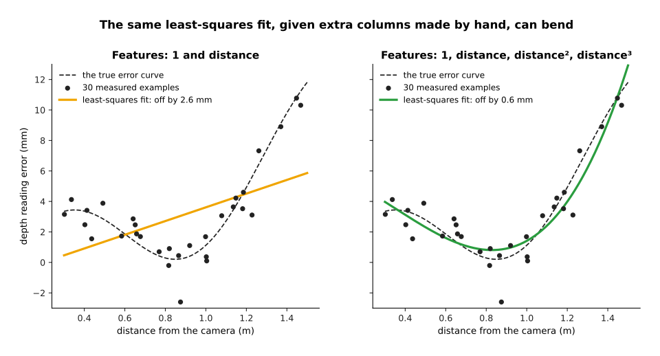
With the features 1 and distance, the fit is a straight line, and it is off by 2.56 mm. Adding distance squared brings this down to 0.65 mm, and adding distance cubed as well brings it to 0.59 mm. Nothing about the method changed in any of this, because only the columns of the table changed.
Choosing features by hand is where most of the skill in linear regression lies, because good features come from knowing the physics. For example, for a joint's friction a person might add the sign of the speed as a feature, because friction pushes against the motion. For a camera lens, the distance from the picture's centre squared is a common feature, because lens bending grows that way.
Ridge regression: a penalty on big weights#
More features let the curve bend more, but with too many features for the number of examples it bends wildly to pass through every noisy point. That is overfitting, and the sign of it here is that the weights become huge and cancel each other out.
Ridge regression fixes this with one change, because it adds a penalty to the thing being made small: the sum of the squared weights, times a number called lambda (λ). The fit must now balance two wishes, which are to stay close to the examples and to keep the weights small. The constant is not penalised, because shrinking it would only move the whole curve up or down.
For example, the script gave 12 examples to a curve with 10 weights, which are powers of the distance up to the ninth. With no penalty, the largest weight is 1,288, and the curve is off by 16.6 mm. With a very small penalty, λ = 0.000001, the largest weight is 422 and the curve is off by 4.2 mm, which is still wild between the examples.
How big should λ be? You cannot use the true curve here, because in real life you do not have it. Instead you use leave-one-out checking, which means leaving out one example, fitting on the other eleven, and seeing how far off the prediction for the left-out one is. Then do this for each of the twelve examples in turn and average the results, and keep the λ with the lowest average.
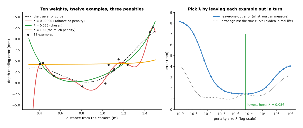
Leave-one-out checking picked λ = 0.056, whose fit is off by 1.39 mm against the true curve and whose largest weight is 6.1. But with λ = 100 the penalty is too strong, so the curve is almost flat and it is off by 3.2 mm. The dotted line on the right, which you would not have in real life, shows that the check picked a good value. Notice the left end of the chosen curve, where there are no examples below 0.4 metres, so the curve rises where it has no data. This means ridge regression only keeps a curve calm between the examples, and not beyond them.
Weighted least squares: trusting some readings more#
Plain least squares treats every example as equally reliable, but often the examples are not equally reliable. For example, a depth camera is less accurate far away than close up, and a force reading taken while the arm is moving has more noise than one taken with the arm still.
Weighted least squares gives each example a weight of its own, and it makes the sum of weight × residual² as small as possible. A reading with a big weight pulls the line hard, while a reading with a small weight pulls it only gently. The usual choice is weight = 1 / (the reading's noise)², so a reading that is 5 times less noisy gets 25 times the say. If you do not know the noise you can measure it, by repeating a few readings at the same load and seeing how much they vary.
So the example calibrates the force sensor again, this time with 30 readings. Twenty were taken with the arm still, which gives a noise of about 0.2 N, but only with light loads, below about 600 counts. Ten were taken while the arm moved, which gives a noise of about 1 N, but they cover the whole range of loads.
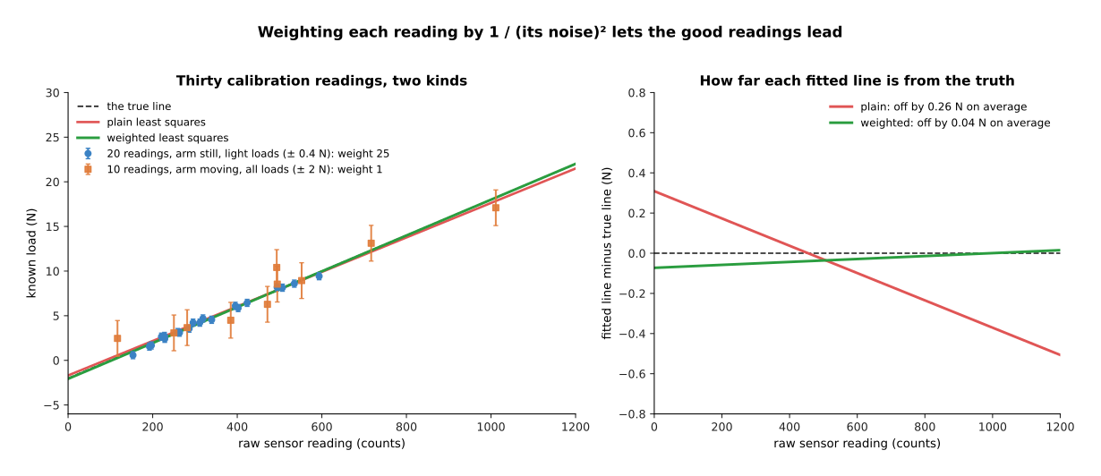
The still readings get weight 25 and the moving ones weight 1. In this run, the plain fit's line is off by 0.26 N on average across the range, and the weighted fit's line by 0.04 N. The right-hand picture shows why, because the plain line is tilted by the noisy readings, and it is worst at high loads, where it matters most.
One run can be lucky, so the script repeated the whole test 2,000 times with fresh noise. On average the plain fit was off by 0.246 N and the weighted fit by 0.117 N. Using only the 20 still readings gave 0.123 N, so weighting did better than both of the alternatives. That is because weighting trusts the still readings most, but it still uses the moving ones to learn about high loads.
Weighting is not special to this page, because the same idea comes back in decision trees and forests, where some examples count more when a tree is built, and in nearest neighbours and locally weighted regression, where closer examples count more.
3. Logistic regression: the chance of a yes#
Everything so far predicted a number, but many questions on a robot have a yes-or-no answer instead. Will this grasp hold? Is this part faulty? Did the peg go into the hole? These are called classification questions, and the answer to one of them is a class. Linear regression is a poor fit for them, because the script fitted a straight line to 200 grasps labelled 1 for held and 0 for dropped, and its outputs ran from −0.03 to 1.40. Neither of those two numbers is a sensible chance, because a chance has to lie between 0 and 1.
Logistic regression keeps the weighted sum, which it now calls the score, and passes it through an S-shaped curve called the logistic function, or sigmoid:
chance = 1 / (1 + e^(−score))
A score of 0 gives a chance of 0.50, while a large positive score gives a chance close to 1 and a large negative score gives a chance close to 0. So the output is always a chance between 0 and 1.
For example, a robot deciding how hard to squeeze has logged 200 past grasps. Each one has two features, which are the grip force in newtons and the width of the object in millimetres. The label is whether the object stayed in the gripper while the arm lifted it. In this simulation more force helps and a wider object is harder to hold, and 135 of the 200 grasps held.
Training uses gradient descent, which the page on how a model learns explained. The measure of how wrong the model is, called the loss, is the log loss. For a grasp that held, the loss is minus the log of the chance the model gave to "held". For a grasp that dropped, it is minus the log of the chance it gave to "dropped", so a confident wrong answer costs a lot. There is no one-step formula here as there is for linear regression, but the loss has a single lowest point, so gradient descent always finds the same answer. The features are first scaled to a similar size, so that one step size suits all the weights.
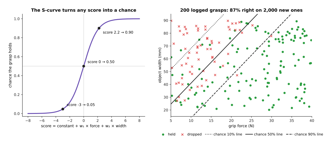
The learned score is 0.67 + 0.264 × force − 0.081 × width, and on 2,000 new simulated grasps it said the right answer, held or dropped, 87% of the time. The lines on the right picture are where the chance is 10%, 50% and 90%. They are straight, because a fixed chance means a fixed score, and a fixed weighted sum is a straight line.
So the robot can now use the model before it acts. The table below gives the chance of holding for three grasps, and you should read each row across: the force, the width, the score and the chance.
| Grip force | Object width | Score | Chance it holds |
|---|---|---|---|
| 20 N | 40 mm | 2.72 | 0.94 |
| 20 N | 70 mm | 0.30 | 0.57 |
| 30 N | 70 mm | 2.94 | 0.95 |
For a 70 mm object, the model says that 27.2 N gives a 90% chance of holding. The weights are also easy to read, because each extra newton adds 0.264 to the score and each extra millimetre of width takes away 0.081. So about 3 mm of extra width needs about 1 N of extra force to make up for it.
Features chosen by hand matter here too, because with grip force alone the model was right 80.3% of the time on the new grasps, against 87.0% with width added. This means the width column carried information that force alone could not give. When there are more than two classes, such as "held", "slipped" and "dropped", the same idea gives each class its own score. Then a function called softmax turns those scores into chances that add up to 1.
4. How they are trained, and how much data they need#
Both methods have been shown on one worked example each, so this section says what they need in general. Both learn from a table, where each row is one example and each column is one feature, plus one more column for the label. You make the features yourself, from measurements that already mean something, such as a distance, a force or a temperature.
Linear and ridge regression are trained in one step, by solving a small set of equations, so training takes well under a second even for a million rows. Logistic regression instead takes a few hundred to a few thousand steps of gradient descent, which is still under a second for tables of this size.
So a rough rule for how much data you need is at least ten examples per weight. The force sensor had 2 weights and 5 examples, which worked because the readings were clean and the true shape really was a line. The ridge example had 10 weights and only 12 examples, which is why it needed a penalty. For logistic regression you should count the rarer class rather than the rows, because if only 20 of your 500 grasps dropped, the model has 20 examples of dropping to learn from and not 500.
Always keep some examples back for checking, as leave-one-out checking does, or split off a test set, because a fit that looks perfect on its own examples can still be wrong between them.
5. Where they are used on a robot arm#
Section 4 showed how little data these methods need, and because they are also small, fast and easy to check, they appear in many places on an arm.
- Sensor calibration. Linear regression turns a force sensor's counts into newtons, a temperature reading into a correction, or a depth camera's reading into the true distance, and this page's two examples are both of this kind.
- Learning an arm's dynamics. The torque a joint needs is a weighted sum of known features built from the joint's angles, speeds and accelerations, where the weights are the links' masses and friction numbers. Finding the weights from logged motion is linear regression, often weighted, because some recorded motions are more reliable than others. Book 6's arm dynamics page describes the formula.
- Predicting grasp success from a few numbers. As in this page's example, logistic regression on force, width, mass or approach angle gives a quick chance that a grasp will hold.
- A small head on a big network. A pretrained network turns each picture into a list of numbers, and a logistic regression then learns the robot's own classes on top of those numbers, from a few dozen labelled pictures. This is called a linear probe, and the fine-tuning page covers it.
- Correcting a physics formula. A formula predicts most of what happens, and a small linear regression learns what it gets wrong, as described in learned dynamics models.
- Simple fault checks. A logistic regression on motor current, temperature and speed gives a chance that a joint is running abnormally.
- A baseline. Before training anything bigger, people fit a ridge or logistic regression first, because if the big model cannot beat it, the big model is not worth its cost.
6. What goes wrong#
Section 5 listed the jobs these methods do well, and this section lists the ways they fail instead. Each failure has a sign that you can look for, and the table below collects them. Read each row across: what goes wrong, the sign you would see, and what people do about it.
| What goes wrong | The sign you would see | What people do about it |
|---|---|---|
| the features cannot draw the true shape | the error stays high however much data you add; the residuals show a pattern, such as all positive in the middle | add features by hand, or move to decision trees and forests or Gaussian processes |
| too many features for the examples | tiny error on the examples, large error on new ones; very large weights | ridge regression, with λ chosen by leave-one-out checking |
| features of very different sizes | the penalty shrinks some weights much more than others; gradient descent is slow | scale every feature to a similar size first |
| two features carry the same information | the weights jump around between fits and have opposite signs | drop one of them, or use ridge regression |
| a few bad readings | the line tilts towards them | weighted least squares if you know which readings are poor; RANSAC from Book 5 if you do not |
| a new input beyond the examples | the prediction runs off, as the ridge curve did below 0.4 m | collect examples there, or refuse to predict outside the known range |
| the two classes are perfectly separated (logistic) | the weights keep growing as training goes on | add a ridge penalty, which scikit-learn does by default |
| a rare class (logistic) | the model says "no" almost every time and still looks accurate | weight the rare class's examples more, and judge the model on the rare class |
7. Libraries#
You would not write any of this from scratch in a real project, so the table below lists real libraries for these methods. Read each row as one library: its language, what it provides, and a note on when to use it.
| Library | Language | What it provides | Note |
|---|---|---|---|
| NumPy | Python | numpy.linalg.lstsq and numpy.linalg.solve | enough for linear, ridge and weighted least squares in a few lines |
| scikit-learn | Python | LinearRegression, Ridge, RidgeCV and LogisticRegression in sklearn.linear_model; PolynomialFeatures and StandardScaler in sklearn.preprocessing | the place to start; fit takes a sample_weight argument for weighting; RidgeCV chooses λ for you |
| statsmodels | Python | OLS, WLS and Logit | prints each weight with an error bar, which helps when you want to read the weights |
| Eigen | C++ | least-squares solvers on matrices | for fitting inside a robot's C++ control code |
scikit-learn's LogisticRegression adds a ridge penalty by default, and its
setting for it is called C, where a smaller C means a stronger penalty.
8. Why these, and what they cost#
The libraries make these methods cheap to try, but the question is still when to choose them. These are the simplest learned models there are, and they turn a table of measured numbers into a number or a chance, using a weighted sum of features that you choose.
What they do for you: they train in under a second, they need few examples when the features are good, and you can read every weight. A weight of 0.264 per newton means something that a person can check, and the residuals show you where the fit is wrong.
The obvious alternative is a small neural network, which does not need you to make features by hand because it learns its own. But with a picture as the input, that difference is decisive. But with a few measured numbers and tens or hundreds of examples, a network needs more examples to reach the same error, has many more settings to choose, and gives weights that nobody can read. The chapter overview shows ridge regression matching a small network on the depth camera problem at every dataset size.
What they cost:
- They can only draw the shapes that their features allow, so finding good features takes both knowledge of the problem and time.
- Logistic regression draws a straight dividing line between the classes, in the space of its features, so a curved boundary needs curved features or a different method.
- They cannot read pictures, point clouds or sound directly, because someone, or some network, must first turn the input into a short list of meaningful numbers.
- Plain linear regression gives no error bar with each prediction, and the Gaussian process page covers a method that does.
9. The written alternative#
Section 8 compared these methods with a neural network, but the closer competitor is a formula that somebody wrote by hand. Book 6's least-squares fitting is the same maths used for a different purpose, which is fitting a shape whose formula is known, such as a plane or a circle, to measured points. Book 6's system identification finds the numbers in a physics formula, such as a motor's gain or a joint's friction, from logged motion, which is linear regression with features chosen by the physics. The written way wins when you know the formula, because then the features are exact and only a few numbers are unknown. Instead, linear regression as a learning method takes over when you only suspect the shape, and try several features to see which ones help. For yes-or-no questions, the written alternative is a hand-set threshold, such as "the grasp is safe if the force is above 25 N". So logistic regression is what you use when two or more numbers matter together and you want the threshold learned from logged results.
10. Where to read next#
- The next page is decision trees and forests, where trees find their own features and handle columns in very different units.
- Gaussian processes and Bayesian optimisation gives a curve with an error bar at every point.
- Nearest neighbours and locally weighted regression fits a small weighted line around each new input, instead of one line for all.
- The chapter overview compares all the methods of this chapter on one table.
- Uncertainty and confidence explains how a robot should use a chance, such as logistic regression's, to decide whether to act.
- Least-squares fitting in Book 5 goes through the maths of the fit in more detail.
11. Using it in Python#
Section 2 worked the weights of a line out from the readings, and section 7 listed the libraries that do it for you. This section joins the two, by showing the calls that produce everything this page described. After reading it you will be able to calibrate a sensor and predict a chance from a table of readings, without writing any of section 2's arithmetic.
from sklearn.linear_model import LinearRegression, Ridge, LogisticRegression

# counts has one row per reading and one column per raw sensor count.
# newtons holds the true force, measured with weights of a known mass.
line = LinearRegression().fit(counts, newtons)
print(line.coef_, line.intercept_)   # section 2's weights and its offset

# alpha is section 2's penalty. A larger alpha pulls the weights harder to zero.
ridge = Ridge(alpha=1.0).fit(counts, newtons)

# trust holds one weight per reading, which is section 2's weighted least squares.
weighted = LinearRegression().fit(counts, newtons, sample_weight=trust)

# slipped holds 1 if that grasp slipped and 0 if it held.
grip = LogisticRegression(C=1.0).fit(X, slipped)
print(grip.predict_proba(X_new)[:, 1])   # section 3's chance of a slip
The column index [:, 1] on the last line is there because predict_proba
returns one column per class, and column 1 is the chance of the class labelled 1,
which here is a slip. Section 7 already warned about the other detail worth
remembering, which is that LogisticRegression applies a ridge penalty by
default and its strength is set by C, where a smaller C means a stronger
penalty. That is the opposite direction from Ridge, where a larger alpha
means a stronger penalty.
The library gives you the solving. LinearRegression finds the exact
least-squares answer, and LogisticRegression runs the iterative fit of section
4, so you never write the normal equations or a gradient. It also gives you
RidgeCV, which tries a list of penalties and keeps the best by
cross-validation.
What you have to collect is the pairs. For the force sensor of section 2 that means physically hanging known weights on the gripper and recording the counts, and no library can do that part. For the slip model of section 3 it means recording grasps and writing down which ones slipped.
What you have to decide is the columns. If the sensor response bends, you add the
bent columns yourself with PolynomialFeatures from sklearn.preprocessing, as
section 2 described, because LinearRegression fits a straight relationship in
whatever columns you hand it. You also decide the penalty, and whether to scale
the columns first, which matters for any penalty because the penalty treats all
weights alike and a column measured in millimetres gets a very different weight
from the same column measured in metres.