This page explains the learning methods that answer a new question by looking up the most similar stored examples. k-nearest neighbours copies the answers of the few closest examples, while weighted neighbours lets the closer ones count more. Locally weighted regression fits a small straight line around each new question, using only the examples nearby. These methods are old and simple, and they are still used on robot arms, from choosing a grasp to learning the arm's own dynamics while it moves.
It answers six questions, and the sections below take them in turn. How do these methods predict a class or a number? Why does weighting the neighbours help? How does locally weighted regression work, and why was it the classic way to learn an arm's dynamics online? Why do the methods fail when each example has many numbers? How can the distance to the nearest examples warn that a new input is unfamiliar? And where does a robot arm use them?
It is for a reader who has read the first chapter of this book, especially how a model learns. So you need to know what an example, a label, a test set and overfitting are.
Every number on this page comes from a real run of the diagram script
docs/diagrams/classical_ml_3.py. The data is simulated, so that the true
answer is known exactly. But the methods themselves are real, and they are
written in NumPy.
Before this page, it helps to have read nearest-neighbour search in Book 5. It explains how a program finds the closest stored points quickly, which every method on this page needs.
Contents#
- The idea in one sentence
- k-nearest neighbours, step by step · Classification: a vote among the nearest · Weighted neighbours: closer ones count more · Measuring distance: units matter
- Regression, and locally weighted regression · A small line around each query · LWPR: learning an arm's dynamics online
- The curse of dimensionality
- Checking for unfamiliar inputs by distance
- How it is trained, and how much data it needs
- Where it is used on a robot arm
- What goes wrong
- Libraries
- Why this, and what it costs
- The written alternative
- Where to read next
- Using it in Python
1. The idea in one sentence#
To answer a new question, find the stored examples whose inputs are most like it, and combine their answers, giving the closest ones the most say.
For example, you want to guess what a house will sell for. You do not write a formula for house prices, so instead you find the five houses that sold most recently on the same street, of about the same size, and take the middle of their prices. If one of them is right next door and nearly identical, you trust it more than the others, and that is k-nearest neighbours with weighting.
2. k-nearest neighbours, step by step#
Section 1 said the method combines the answers of the most similar examples, so this section says exactly how. k-nearest neighbours (kNN) does no training at all, because it simply keeps every example. To answer a new input, called the query, it:
- measures the distance from the query to every stored example's input;
- takes the k examples with the smallest distances, the neighbours;
- combines their labels: a vote for a class, or an average for a number.
k is a number that you choose, such as 5, and step 1 is the slow part when there are many examples. So Book 6's nearest-neighbour search builds a k-d tree, a structure that finds the neighbours without measuring every distance.
Classification: a vote among the nearest#
For example, an arm has logged 150 grasps, and each grasp has two input numbers: the object's width in millimetres (mm), and how far the grasp was to one side of the object's centre, the offset, also in mm. The label says whether the grasp held or slipped. In this simulation a grasp holds if the offset is small enough for the width, because wide objects leave less room. To make it realistic, 8% of the labels were flipped, as if some grasps failed for reasons the two numbers do not show.
Take one query, a 60 mm object grasped 12 mm off centre, whose five nearest logged grasps are between 3.1 and 3.8 mm away. Three of them held and two slipped, so the vote is 3 to 2 and kNN predicts "holds". The truth, from the rule, is also "holds".
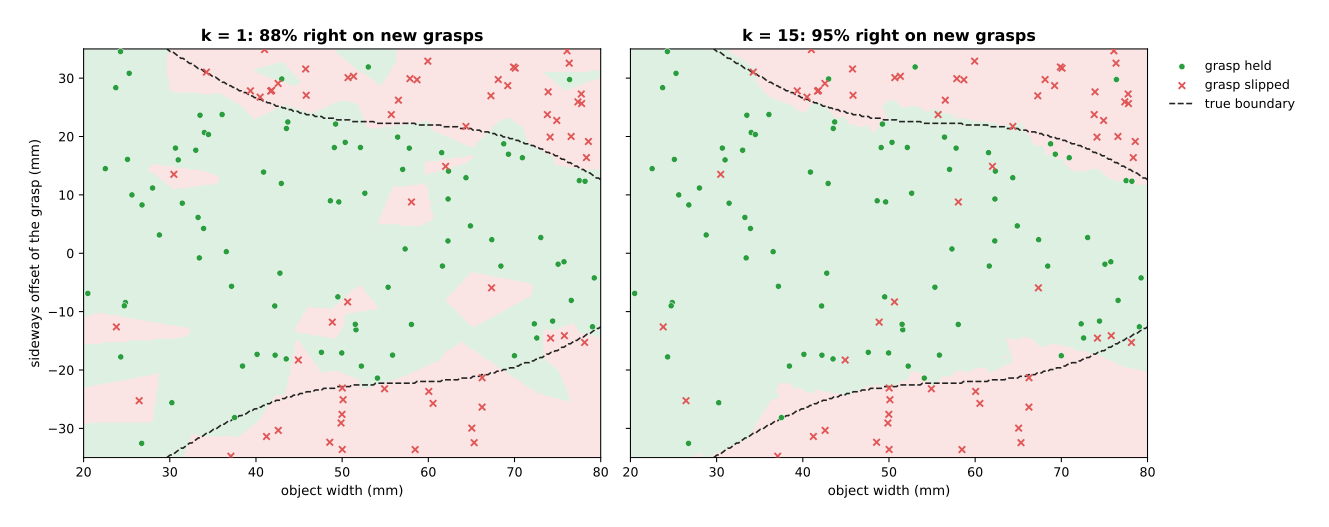
The picture shows the answer kNN gives at every point, where green means "holds" and red means "slips". The dashed line is the true boundary, and the script scored each setting on 4,000 new grasps.
- With k = 1, every flipped label makes its own island of the wrong colour, so it is right only 88% of the time.
- With k = 15, the islands vanish, because one wrong label is outvoted, and it is right 95% of the time.
A larger k smooths the answer, but too large a k smooths away real detail, because with k = 45 the vote reaches so far that it is right only 86% of the time. So k is chosen by trying several values on examples held back for testing.
Weighted neighbours: closer ones count more#
In a plain vote the 15th neighbour counts as much as the first, even if it is ten times as far away, so weighted neighbours gives each neighbour a weight that falls with its distance. The most common weight is one divided by the distance, so a neighbour 2 mm away counts five times as much as one 10 mm away. The answer is then the weighted vote, or the weighted average.
The table below compares plain and weighted votes on the same 150 grasps. Read each row across: k, then how often each kind of vote was right on 4,000 new grasps.
| k | Plain vote | Weighted vote |
|---|---|---|
| 1 | 88.3% | 88.3% |
| 5 | 95.6% | 95.0% |
| 15 | 94.6% | 96.8% |
| 45 | 86.0% | 95.0% |
With k = 1 the two are the same, because there is only one neighbour. With a small k weighting changes little, but with a large k it matters a lot. At k = 45 the plain vote lets far examples outvote near ones, while the weighted vote gives them little say and stays at 95%. So weighting makes the choice of k much less delicate.
Measuring distance: units matter#
The usual distance is the straight-line distance, which means squaring the difference in each input, adding them up, and taking the square root. This treats one unit of every input as equally important, so it is only fair if the units are comparable.
In the grasp example both inputs are in millimetres, and kNN with k = 5 is right 95.6% of the time. The script then gave the width in metres instead, while keeping the offset in millimetres. Now a 60 mm difference in width counts as 0.06, while a 1 mm difference in offset counts as 1. So the distance almost ignores the width, and kNN is right only 82.8% of the time.
The fix is to standardise each input before measuring distance, which means subtracting its average and dividing by its spread. With both inputs standardised kNN is right 95.1% of the time. So always do this when the inputs have different units, such as a joint angle in radians and a force in newtons.
3. Regression, and locally weighted regression#
Section 2 voted among the neighbours to get a class, and for a number instead kNN averages the neighbours' labels. In the robot example a joint's friction torque, in newton metres (N m), depends on its speed, in radians per second (rad/s). The robot has 40 measurements at speeds from −1 to 1 rad/s, each with noise of 0.04 N m.
Plain kNN with k = 6 averages the six nearest measurements, while weighted kNN weights them by one over the distance, and the right panel below shows both. Plain kNN draws a staircase, because the answer jumps whenever the set of six neighbours changes. Weighted kNN is smoother, but it bends towards each single measurement, noise and all.
A small line around each query#
Locally weighted regression (LWR) goes one step further, because for each query it fits a straight line, but only to the examples near that query. It does this with weighted least squares, which the regression page explains: each example gets a weight, and the line fits the heavy examples most closely.
- Give every example a weight that falls with its distance from the query. Here the weight has a bell shape with a width of 0.12 rad/s. So an example 0.12 rad/s away gets weight 0.61, one 0.24 away gets 0.14, and one 0.36 away gets 0.01.
- Then fit a straight line to all the examples, using those weights, so that far examples have almost no say.
- Then read the line's value at the query, and that value is the prediction.
- For the next query, start again with new weights.
So LWR is not one model, because it is a new small model for every query. The line also lets it follow a slope, which an average cannot do.
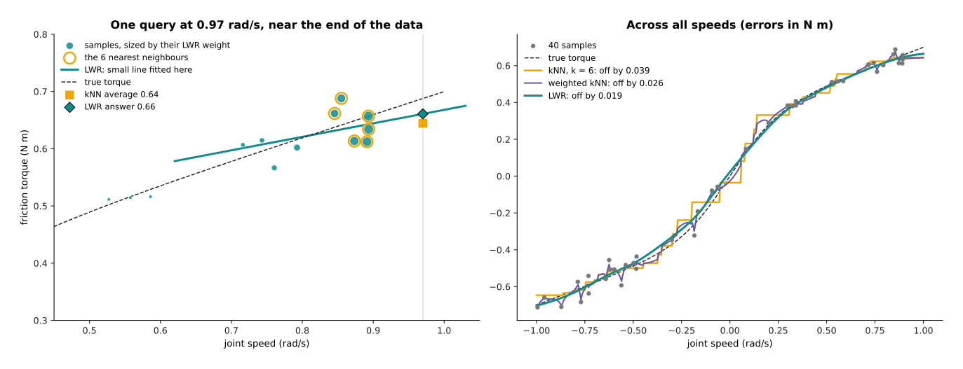
The left panel shows one query, at 0.97 rad/s, where each dot's size shows its LWR weight. The true torque there is 0.688 N m, and the six nearest measurements all lie to the left of the query, between 0.85 and 0.89 rad/s. Their average is 0.644 N m, which is too low, because the torque rises with speed and every neighbour sits at a lower speed. Weighted kNN gives 0.642, for the same reason. But LWR fits a line through the nearby measurements and follows it out to 0.97, so its answer is 0.661 N m, which is closer to the truth. Its line rises by 0.24 N m for each rad/s, flatter than the true 0.40, because a few noisy measurements pull it. So it closes part of the gap, not all of it.
The table below scores the three methods against the true curve. Read each row across: the method, its average error over all speeds, and its average error near the two ends of the data, above 0.85 rad/s in either direction.
| Method | Error overall | Error near the ends |
|---|---|---|
| kNN, k = 6 | 0.039 N m | 0.030 N m |
| Weighted kNN, k = 6 | 0.026 N m | 0.030 N m |
| LWR, width 0.12 rad/s | 0.019 N m | 0.016 N m |
LWR has half the error of plain kNN overall, and half the error near the ends. The ends are where an average suffers most, since all of its neighbours lie on one side.
The width plays the part that k plays in kNN. A narrow width follows every bump, including noise, while a wide width smooths away real bends. So it is chosen by testing several widths on held-back examples.
LWPR: learning an arm's dynamics online#
An arm's inverse dynamics is the torque each joint needs to make a given motion. Book 6's arm dynamics computes it from a physics formula. For a seven-joint arm the input is 21 numbers, which are the angle, speed and acceleration of each joint, and the output is seven torques. The formula misses friction, cables and wear, so researchers in the late 1990s and 2000s set out to learn this mapping from the arm's own motion, while it moved.
But plain LWR is too slow for that, because it fits a new line for each query from all the stored examples. So locally weighted projection regression (LWPR), published by Sethu Vijayakumar, Aaron D'Souza and Stefan Schaal in 2005, was the classic answer, and it works like this.
- It keeps a set of local models, where each one has a centre, a region it covers, and a small linear fit that is valid only in that region.
- When a new measurement arrives, every local model near it updates its fit a little. The measurement is then thrown away, so that memory does not grow with time.
- If no local model covers the new measurement well, LWPR creates a new one centred there.
- Each model also adjusts the size of its region: smaller where the mapping bends fast, larger where it is nearly flat.
- To predict, it takes the answers of the local models near the query and averages them, weighted by how well each one covers the query.
The word "projection" refers to one more trick. Within each region, LWPR finds the few directions among the 21 inputs along which the output actually changes, and it fits its line only along those. Real arm motion covers only a thin slice of all possible 21-number inputs, so a few directions are usually enough, and that is how LWPR avoids the problem of the next section.
LWPR learned the dynamics of real research arms, such as the seven-joint SARCOS arm, in real time, and later work used local Gaussian processes the same way. Today a small neural network, trained on logged data, often does this job, as in this book's learned arm models. LWPR's idea of learning online, from local pieces that do not disturb each other, is still useful when an arm must adapt while it works.
4. The curse of dimensionality#
Section 3 used one input number, and nearest-neighbour methods work well with a few. With many of them they fail, for a reason that has a famous name: the curse of dimensionality, where each input number counts as one dimension.
In plain words, as you add input numbers, the space grows so fast that the stored examples become spread thinly, and every example ends up far from every other. So the "nearest" neighbour is then not near at all, because it is only a little nearer than the rest.
The script shows this with 2,000 random examples, spread evenly, and 200 random queries, for 1 to 30 dimensions.
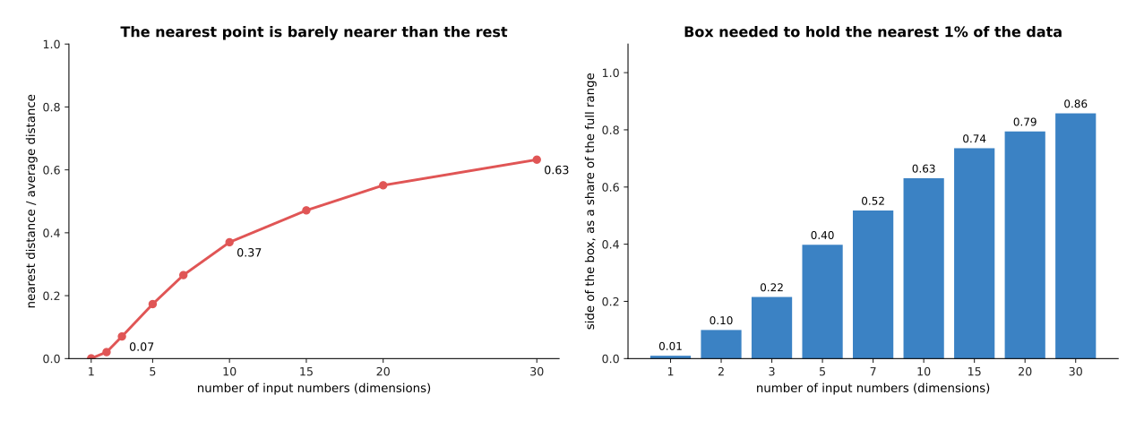
The left panel divides the distance to the nearest example by the average distance to all examples. In 2 dimensions this is 0.02, which means the nearest example is fifty times closer than a typical one. But in 10 dimensions it is 0.37, and in 30 dimensions it is 0.63. So the nearest example is then almost as far as any other, and copying its label means little.
The right panel shows the same problem another way. To gather the nearest 1% of the examples inside a box, the box must span 10% of each input's range in 2 dimensions, while in 10 dimensions it must span 63% of each input's range. So the "neighbourhood" then covers most of the space, and it is no longer local.
On a robot this means using neighbours on a few carefully chosen input numbers, such as an object's width and weight, rather than on raw pixels. Real data helps a little, because it usually lies on a thin slice of the space, as LWPR used. So a common trick is to let a neural network turn a picture into a short list of numbers first, and then search for neighbours among those.
5. Checking for unfamiliar inputs by distance#
Section 4 showed that distance loses its meaning with many inputs, but with a few inputs distance is useful in its own right. Any learned model can give a confident wrong answer for an input unlike its training examples, and such an input is called out of distribution. So the distance to the nearest training examples gives a simple check: if a new input is far from all of them, the model has not seen anything like it, and its answer should not be trusted.
For example, a model predicts a correction torque from two joint angles. It was trained on 300 poses from the arm's usual work, which fill a curved band of angles, but the robot then meets poses from anywhere in the range.
To set a limit, the script first measures, for each training pose, the distance to its nearest other training pose. Inside the data the typical value is 0.030 radians (rad), and 99% of them are below 0.133 rad. So the check uses 0.133 rad as its limit, which means a new pose farther than that from every training pose is flagged.
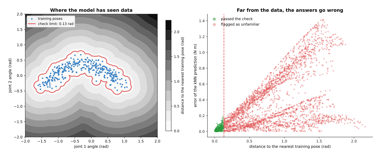
The left panel shades each point by its distance to the nearest training pose, and the red line is the limit. The right panel then tests 3,000 random poses, and it plots the error of a kNN prediction against the distance to the nearest training pose.
- 13% of the test poses passed the check, and their average error was 0.031 N m, so only 4.2% of them had an error above 0.1 N m.
- The other 87% were flagged. Their average error was 0.393 N m, and 79% of them had an error above 0.1 N m.
So the check caught most of the bad answers and let through mostly good ones, and the robot can then refuse to use the correction, move more slowly, or ask a person.
The check works for any model and not only for kNN. For a neural network, measure the distance between the network's internal numbers for the new input and for the training inputs, instead of between the raw inputs. The uncertainty and confidence page covers other ways to tell when a model is unsure.
6. How it is trained, and how much data it needs#
Section 5 used stored examples as a check rather than as a model, and this section says what storing them costs. kNN is not trained at all, because "training" means storing the examples and building a search structure such as a k-d tree if there are many. Adding a new example is instant, since it is simply stored, and that makes kNN a natural fit for a robot that learns as it works.
You still choose a few things: k, or the LWR width; the weighting; and how to scale each input. So choose all of them by testing on held-back examples.
How much data you need depends on the number of inputs. With one or two inputs, tens of examples give useful answers, as in the friction example with 40. But every extra input needs many more examples to keep the neighbours near, as section 4 showed. So beyond about 10 raw inputs, kNN usually does poorly unless the data lies on a thin slice.
The examples must also cover the inputs the robot will meet, because kNN cannot guess beyond its data. Far from all examples it still returns the labels of the nearest ones, however far away they are, and that is why the distance check matters.
7. Where it is used on a robot arm#
Section 6 said these methods suit a robot that keeps learning while it works, and six jobs on an arm look like that. Reusing what worked. A robot keeps a store of objects it has grasped, holding a few numbers describing each object's shape and the grasp that worked. For a new object it finds the most similar stored object and tries its grasp first. This is kNN with k = 1, and it is one of the most common learning methods on real arms.
Predicting whether a grasp will hold. This is the example in section 2, where a few numbers about the object and the grasp lead to a vote among similar past grasps.
Learning the arm's dynamics online. This is LWR and LWPR, as in section 3, where a learned correction torque is added to the physics formula's torque as feed-forward.
Choosing an action from demonstrations. A robot stores the camera view and the action at each moment of some demonstrations. Then at run time it finds the stored moments most like the current view, and averages their actions. The VINN method, published in 2021, did this with a neural network's summary of each picture, and did about as well as more complex learners in its tests.
Flagging unfamiliar inputs. This is the check in section 5, placed in front of any other model, from a friction correction to a grasp network.
Finding the stored scene most like the current one. For example, matching the current pose of a part to a library of stored poses, each with a known pick plan.
8. What goes wrong#
Section 7 listed where these methods work, and seven things go wrong often enough to be worth looking for. Inputs in different units. One input with large numbers swamps the rest, as the metres-and-millimetres test showed. So standardise every input before measuring distance.
Too many inputs. This is the curse of dimensionality, so choose a few meaningful inputs, or let a network reduce a large input to a short one first.
Noise in single examples. With k = 1 every wrong label is copied, so use a larger k and weight the neighbours.
Answers at the edge of the data. An average of neighbours that all lie on one side is biased, as the query at 0.97 rad/s showed, and LWR's local line reduces that bias.
Far from all data. kNN always answers, even when the nearest example is far away, so add the distance check in front of it.
Slow answers with many examples. Measuring every distance is slow for millions of examples, so use a search structure, such as a k-d tree, or an approximate search library.
Memory. kNN stores every example, so on a small robot computer a store of camera pictures fills memory fast. Store short summaries instead, or keep only a chosen subset of the examples.
9. Libraries#
You would use a library rather than write the search yourself, and these are the real ones that provide the methods on this page.
- scikit-learn:
KNeighborsClassifierandKNeighborsRegressor, both withweights='distance'for weighted neighbours;NearestNeighborsfor the search on its own, which is useful for the distance check; andStandardScalerto standardise inputs. - FAISS, from Meta: fast nearest-neighbour search over millions of examples, exact or approximate, with graphics-card support.
- statsmodels: a
lowessfunction, which is locally weighted regression for one input. - The LWPR library, from the authors of LWPR: written in C, with interfaces for C++, MATLAB and Python.
But kNN and LWR are also short enough to write yourself, and the script behind this page does each of them in a few lines of NumPy.
10. Why this, and what it costs#
Those libraries make these methods cheap to try, so this section answers the four questions: what it is, what it does for you, why it rather than the obvious alternative, and what it costs.
kNN and LWR predict by combining the labels of the stored examples most similar to the query. They need no training, they learn a new example instantly, and every answer can be explained by pointing to the examples it came from.
The obvious alternative is one global model, such as linear regression or a small neural network, which must have the right shape everywhere at once. A straight line cannot follow the friction curve's bend, and a network can, but it must be trained again to take in new examples and it may forget old ones. Instead kNN and LWR fit the shape piece by piece, so a new example changes only the answers near it. So choose them when the inputs are few, the shape is unknown, and the robot keeps learning while it works.
The other alternative is a Gaussian process, which also predicts from nearby examples. A GP gives an error bar, and its curve is smoother. But kNN and LWR stay fast with many more examples, although they give no error bar of their own, and LWPR updates in real time.
The costs are these. You must store every example, or LWPR's local models, and search them at each query, and you must scale the inputs and choose k or the width. The methods also fail with many raw inputs. And they cannot predict beyond their data, because far from every example they still answer, so you must check the distance yourself.
11. The written alternative#
Book 6's nearest-neighbour search is the programmed half of kNN, because it finds the closest stored points exactly. On its own it is a lookup table, where you store the grasps you have tested by hand and look up the nearest one. That wins when a person can list the cases ahead of time and there are few of them. But kNN adds the learned part, which is a vote or a weighted average over several neighbours, so that noise in one example does not decide the answer.
For the arm's dynamics, the written alternative is Book 6's system identification, which fits the numbers in a physics formula. It wins whenever the formula has the right shape, because it needs far fewer examples and it behaves sensibly away from the data. But LWR and LWPR win for effects the formula does not describe, such as friction that changes with pose. So the usual choice is both: the formula first, and a local learner on what it gets wrong.
12. Where to read next#
- The previous page is aussian processes and Bayesian optimisation](03_gaussian-processes-and-bayesian-optimisation.md), where a GP also predicts from nearby examples but adds an error bar.
- Linear and logistic regression explains weighted least squares, the fit inside LWR.
- Learned arm models learns the arm's dynamics with networks, the modern follow-on to LWPR.
- Uncertainty and confidence covers other ways to tell when a model should not be trusted.
- The chapter overview compares all the methods of this chapter in one table.
- Book 6's nearest-neighbour search explains k-d trees and fast search in detail.
13. Using it in Python#
Section 2 looked up the nearest examples by hand, section 5 turned the distance to the nearest example into a check for unfamiliar input, and section 9 named the libraries. This section shows the calls, and there are only three of them, because the method has almost nothing to train.
from sklearn.neighbors import KNeighborsRegressor, NearestNeighbors
from sklearn.preprocessing import StandardScaler
from sklearn.pipeline import make_pipeline

# StandardScaler comes first, because section 2 showed that the units of each
# column decide which examples count as near.
model = make_pipeline(
    StandardScaler(),
    KNeighborsRegressor(n_neighbors=5, weights="distance"))
model.fit(X, y)
print(model.predict(X_new))

# Section 5's check: how far is this input from anything we have seen?
index = NearestNeighbors(n_neighbors=1).fit(X)
distance, _ = index.kneighbors(X_new)
The argument weights="distance" is section 2's weighted vote, where a closer
neighbour counts for more, and leaving it out gives every one of the five
neighbours an equal say. The make_pipeline call matters more than it looks,
because it means the scaling learned from the training rows is applied to
X_new too. Scaling the two sets separately is a common mistake and it quietly
ruins the distances.
The library gives you the search, and it picks a data structure for you. With few columns it builds a k-d tree or a ball tree, which finds the nearest examples without comparing against every row, and with many columns it falls back to comparing against every row, because those trees stop helping. That is section 4's curse of dimensionality showing up inside the library.
What you have to keep is the data, and this is the one method where that is
literal. fit stores the rows and learns nothing, so all the cost moves to
predict, and the saved model is as large as your dataset. If you delete the
training rows you have deleted the model.
What you have to decide is n_neighbors, the scaling, and the distance above
which you refuse to answer. Section 2 explained why the first of those is a real
trade, because a small k follows the noise and a large k smooths over real
detail. The refusal limit of section 5 has no default at all, and you set it the
way section 5 did, by measuring how far each training example sits from its
nearest neighbour and taking the value that 99% of them fall below. For the
locally weighted regression of section 3 with a single input column,
statsmodels has a lowess function, which scikit-learn does not provide.