This page explains principal component analysis (PCA). PCA looks at a pile of examples, each made of many numbers, and finds the few directions in which the examples differ most. So keeping only those directions turns each example into a few numbers instead of many. The page answers five questions, and the sections below take them in turn. What does PCA find? How does it find it? How many directions should you keep? Where does a robot arm use it? And what goes wrong?
It is for a reader who has read chapter 1 of this book, in particular what a model is and how a model learns. So you need to know what an example is, although you do not need labels for this page, because PCA learns from examples alone.
Before this page, it helps to have read planes: the singular value decomposition in Book 5. That section finds the directions in which a set of 3D points spreads out. PCA is the same calculation, used on any kind of numbers.
Every number on this page comes from a real run of the diagram script
docs/diagrams/classical_ml_5.py. The data is simulated, so that what is hidden
in it is known. But the method itself is real, and it is written in NumPy.
Contents#
- The idea in one sentence
- How it works, step by step
- Keeping a few out of many
- How it is trained
- Where it is used on a robot arm
- Beyond straight directions: t-SNE, UMAP and autoencoders
- What goes wrong
- Libraries
- Why PCA, and what it costs
- The written alternative
- Where to read next
- Using it in Python
1. The idea in one sentence#
PCA finds the directions in which a set of examples varies most, in order from most to least, so that you can describe each example by how far it lies along the first few directions and drop the rest.
For example, people stand in a long, straight queue at a bus stop. To say where each person stands you could give two numbers, which are how far east and how far north. But everyone stands on the same line, so one number is enough: how far along the queue. The second number, how far a person stands to the side of the line, is small and tells you little. PCA finds the line of the queue for you, from the positions alone, and it also works when the "positions" have 15 or 350 numbers instead of two.
The directions PCA finds are called principal components, where the first principal component is the direction of most spread. The second is the direction of most spread that is at right angles to the first, and so on. "Spread" here means how far the examples lie from their average, measured as the variance, which is the average of the squared distances from the mean.
2. How it works, step by step#
Section 1 said PCA finds the directions of most spread, so this section finds them on a small example. The example is a robot hand with a finger of three joints, of which we look at two: the middle joint and the end joint. The hand closes on eight different objects, and each time the program records the two angles in degrees. In a real finger the two joints bend together, so the readings lie close to a line.
| Reading | 1 | 2 | 3 | 4 | 5 | 6 | 7 | 8 |
|---|---|---|---|---|---|---|---|---|
| middle joint | 16 | 27 | 66 | 51 | 17 | 40 | 44 | 21 |
| end joint | 14 | 34 | 52 | 39 | 16 | 31 | 32 | 19 |
Read the table one column at a time: each column is one reading, with two numbers. PCA then runs these steps.
- Find the average of each number. The mean middle angle is 35.2° and the mean end angle is 29.6°, and together they are the centre of the readings.
- Subtract the average from every reading. Now the readings sit around zero, and this step is called centring.
- Measure how the numbers spread together. This gives a small table called the covariance matrix. On its diagonal it holds the variance of each number, which is 323.9 for the middle joint and 165.4 for the end joint. Off the diagonal it holds 218.2, which is large and positive, so that says the two angles tend to go up together.
- Find the directions of that spread. A standard piece of linear algebra,
the eigen-decomposition, turns the covariance matrix into directions and
the variance along each. NumPy does it with
np.linalg.eigh, and here it gives direction 1 = (0.819, 0.574), which points up and to the right at 35.0°, with a variance of 476.9. Direction 2 = (−0.574, 0.819), at right angles to it, has a variance of only 12.5. - Describe each reading by its distance along direction 1. Multiply the centred reading by the direction, number by number, and add them up. The result is called the reading's score, so reading 3, (66, 52), gets a score of 38.0, while reading 1, (16, 14), gets −24.7.
- Rebuild a reading from its score, if you need to. Start at the mean and go the score's distance along direction 1. Reading 3 then comes back as (66.4, 51.4), which is 0.7° from the recorded reading.
The picture below shows the steps. On the left are the readings, their mean and the two directions, where each arrow is twice as long as the spread along it. On the right, each reading is dropped straight onto direction 1, and its score is where it lands.
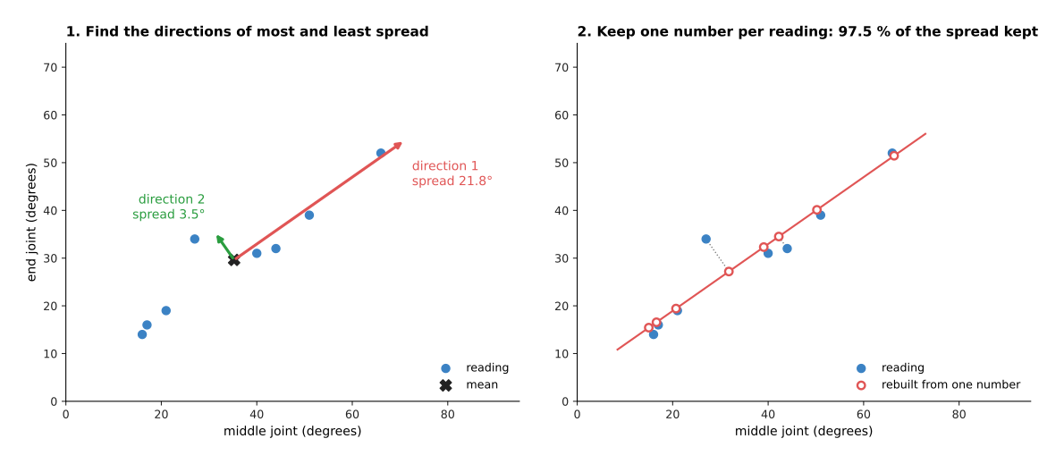
The spread along direction 1 is 21.8°, while the spread along direction 2 is 3.5°. So direction 1 holds 476.9 / (476.9 + 12.5) = 97.5% of the total variance, which means that by keeping one number per reading instead of two, we keep 97.5% of the spread. The rebuilt readings are then 2.2° from the recorded ones on average. The worst one, reading 2, is 8.3° off, because it lies far from the line.
The whole method fits in a few lines of NumPy:
mean = x.mean(axis=0)                     # step 1
centred = x - mean                        # step 2
cov = np.cov(centred.T)                   # step 3
values, vectors = np.linalg.eigh(cov)     # step 4, smallest variance first
order = np.argsort(values)[::-1]          # put the largest first
values, vectors = values[order], vectors[:, order]
scores = centred @ vectors[:, :k]         # step 5: keep k numbers per reading
rebuilt = mean + scores @ vectors[:, :k].T   # step 6
Here x holds one reading per row, and k is how many directions to keep.
3. Keeping a few out of many#
With two numbers PCA saves only one, so it becomes useful when each example has many numbers. The second example is the whole hand, which is five fingers with three joints each, so 15 joint angles per posture. The hand grasps 210 objects, of which seventy are held in a power grasp, with the whole hand wrapped round the object. Seventy more are held in a pinch, between thumb and index finger, and seventy are touched with a flat hand.
In this simulation every posture is made from a resting posture, two hidden patterns and a weak third one, plus 3° of random noise on each joint. But PCA is not told any of this, because it sees only 210 rows of 15 numbers.
PCA gives 15 directions, one for each number, and the picture below shows the share of the total variance that each direction holds, with the running total.
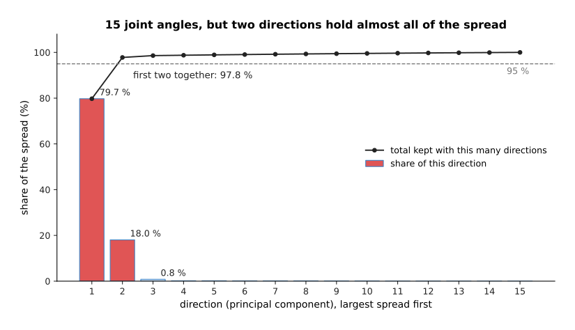
The first direction holds 79.7% of the spread and the second holds 18.0%, so together they hold 97.8%. The third holds only 0.8%, and each of the other twelve holds 0.2% or less, which is the noise.
A common rule is to keep enough directions to hold 95% of the variance, which here is two. Another rule is to look for the elbow, which is the point where the bars drop and then stay low, and here the elbow is after direction 2 as well.
What do the two directions mean? Each direction is a list of 15 weights, one per joint, and the table below gives them. Read each row as one finger, with the weights for its base, middle and end joints.
| Finger | Direction 1 (base, middle, end) | Direction 2 (base, middle, end) |
|---|---|---|
| thumb | +0.26, +0.29, +0.22 | +0.35, +0.36, +0.27 |
| index | +0.26, +0.29, +0.21 | +0.32, +0.35, +0.20 |
| middle | +0.27, +0.29, +0.22 | −0.12, −0.12, −0.13 |
| ring | +0.27, +0.29, +0.22 | −0.23, −0.23, −0.24 |
| little | +0.27, +0.29, +0.22 | −0.25, −0.25, −0.28 |
Direction 1 bends every joint by about the same amount, so it means "close the whole hand". Direction 2 bends the thumb and index finger and straightens the other three, so it means "pinch". In hand research such a pattern of joints that move together is called a synergy, and PCA found both synergies from the postures alone.
Keeping few directions does lose a little. If each posture is rebuilt from one number, the joints are 10.1° wrong on average, measured as the root mean square (RMS) error, which means squaring each error, averaging, and taking the square root. With two numbers the error drops to 3.3°, and with three it is 2.7°, which is about the size of the noise that was added. So more directions would only copy the noise.
4. How it is trained#
Section 3 kept two directions out of fifteen, and this section says what the fitting behind that costs. PCA needs no labels, because it learns from the examples alone, which is why it is called an unsupervised method. Its "training" is the calculation in section 2: find the mean, find the covariance matrix, and find its directions. So there is no repeated nudging of weights and no learning rate, and the answer is the same every time for the same data.
What it learns is the mean and the directions, which for the hand is 15 numbers for the mean and 15 for each kept direction. After that, turning a new posture into its scores is one subtraction and one multiplication.
How much data does it need? More examples than numbers per example is the minimum, because with fewer some directions cannot be found at all. Several times more examples than numbers is a safer start, and the hand used 210 examples for 15 numbers. The examples must also cover the situations the robot will meet, because PCA only finds the directions that it sees.
The calculation is cheap, because for a few thousand examples of a few hundred
numbers it takes well under a second. For very wide data, such as camera
pictures, the program usually uses the singular value decomposition (SVD),
np.linalg.svd, straight on the centred data. This gives the same directions
without building the large covariance matrix first.
One choice matters a lot, and that is the units, because PCA measures spread in the units it is given. If one column is a joint angle in degrees and another is a force in newtons, the column with the larger numbers wins, whatever it means. So the program first standardises each column when the units differ, which means subtracting the column's mean and dividing by the column's spread. Then every column counts equally.
5. Where it is used on a robot arm#
Finding a surface's normal#
Section 4 said PCA is cheap and needs no labels, so it turns up in five different jobs on an arm. A normal is the direction straight out of a surface, and the arm needs it to push a suction cup square onto a box, or to line up a tool with a wall. The program takes a small patch of 3D points from the depth camera and runs PCA on their x, y and z values. The points spread widely in two directions along the surface and hardly at all out of it. So the direction of least spread, which is the last principal component, is the normal.
Book 5 uses exactly this calculation. Iterative closest point finds a normal at every point of a scan from its nearest neighbours, and least-squares fitting fits a whole plane this way, with a real run on 150 points. The same directions taken over a whole object give its long axis and its thin axis, which tells a gripper which way to close. Book 1 shows this for a bar in which way an object lies, and Book 2 fits a box to an object with it in an oriented box round the point cloud.
Compressing joint and force signals#
A recorded movement has many numbers. Take a 7-joint arm that reaches from a home posture to an object, where if each joint is recorded 50 times during the reach, one reach is 7 × 50 = 350 numbers. In this simulation 300 reaches were recorded, and each one goes to a different place on the table and lifts a little over whatever is in the way. But behind each reach there are only four hidden numbers: three for where the object is, and one for how high the lift is. There is also 0.3° of sensor noise on every reading.
PCA was trained on 250 of the reaches and tested on the other 50. The first three directions hold 99.53% of the variance, and the first four hold 99.96%, so the picture below shows one test reach rebuilt from its scores.
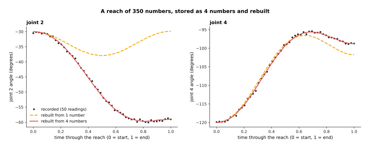
With one number the rebuilt reach is 10.26° RMS off and the worst joint is 82.30° off, because one number cannot say where the object is. With four numbers the error is 0.30° RMS, which is the same as the sensor noise, and the worst reading is 1.33° off. So each reach can be stored or sent as 4 numbers instead of 350. The program must also keep the mean reach and the four directions, but those are stored once, for all the reaches.
The same works for a window of force readings, because a wrist force sensor gives six numbers per reading, so a 100-reading window is 600 numbers. PCA can squeeze such a window into a few scores. The scores then go into a smaller learned model, such as a decision tree that tells "in contact" from "free", or a hidden Markov model that follows the steps of an insertion. So fewer input numbers means the model needs fewer examples to learn.
A few synergies for a many-jointed hand#
Section 3 found that two synergies describe a 15-joint hand well, and a robot can use that the other way round. Instead of controlling 15 joints, the controller sends two numbers: how far to close, and how much to pinch. Each number then moves every joint by its weight in the synergy. This makes a many-jointed hand much easier to drive by a person with a joystick, or by a planner that searches over grasps.
This idea comes from real hands, because a well-known 1998 study by Santello, Flanders and Soechting recorded people shaping their hands to hold many objects. It found that the first two principal components held more than 80% of the variance of the joint angles. Some robot hands are built on that result, and the Pisa/IIT SoftHand closes all its fingers with a single motor, along one synergy.
Looking at a dataset#
People cannot see 15 numbers at once, but they can see two, so plotting each example by its first two scores gives a picture of the whole dataset. The picture below does this for the 210 hand postures, coloured by grasp type.
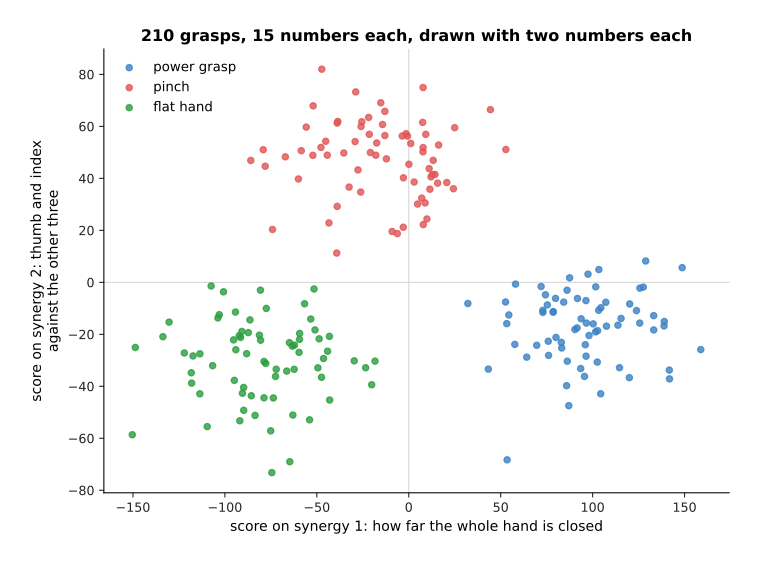
The three grasp types form three separate groups. Power grasps lie to the right, where the hand is most closed, while pinches lie at the top and flat hands lie low and to the left. So such a picture shows at a glance whether the grasp types can be told apart, whether some examples are odd, and whether a new batch of recordings looks like the old one. A Gaussian mixture model could then find the three groups from these two scores without being told the grasp types.
Shrinking the input for another model#
Methods that compare examples by distance, such as nearest neighbours and Gaussian processes, work poorly when each example has hundreds of numbers, because in that many numbers every example is far from every other, and the noise in the unimportant numbers drowns the important differences. So running PCA first, and feeding only the first few scores to the next model, is a common fix.
6. Beyond straight directions: t-SNE, UMAP and autoencoders#
Every use in section 5 relied on straight directions, and PCA only finds straight directions. Some data lies on a curved surface instead, such as the postures of an arm that turns all the way round, and PCA then needs many directions to describe something that has only a few real degrees of freedom. So three other tools are often named next to PCA.
t-SNE, short for "t-distributed stochastic neighbour embedding", and UMAP, short for "uniform manifold approximation and projection", draw each example as a point in two dimensions. They try to keep examples that were close together close in the picture, and they often show groups that PCA's picture hides. But they are for looking only. The distances between groups in their pictures mean little, the picture changes with their settings and with the random start, and they cannot turn a new example into a point without running again. So engineers use them to look at a dataset, and PCA to shrink data inside a running program.
An autoencoder is the learned, curved version of PCA, because it is a neural network with an encoder, which squeezes an example into a short code, and a decoder, which rebuilds the example from the code. Training makes the rebuilt example as close to the original as it can. An autoencoder whose two halves are each one plain weighted sum, with no simple rule after it, learns to keep the same directions as PCA. But with more layers it can follow curved data, and it can squeeze a whole camera picture into a few numbers. This book shows this inside a latent world model, and encoders and decoders explains the two halves. The price is the usual price of a network: many more examples, training that takes a long time, and a code whose numbers have no clear meaning.
7. What goes wrong#
Section 6 named what PCA cannot do, and seven more things go wrong often enough to be worth looking for. Mixed units give the wrong directions. A column in millimetres beats a column in metres, only because its numbers are larger. So the fix is to standardise each column first, as section 4 describes, or to choose units that make the columns similar in size.
Forgetting to centre gives a wrong first direction. Without step 2 the first direction points from zero to the average of the data, rather than along its spread. Libraries centre for you, but code written by hand must do it itself.
A few bad readings pull the directions. One depth point on the wall behind a box can turn the box's normal by several degrees, because PCA squares the distances. So the fix is to remove outliers first, for example with RANSAC, or to fit the normal to a smaller patch.
The largest spread is not always the useful part. PCA keeps what varies most, and not what matters most for the job. For example, if a slip shows up as a tiny ripple in the force signal, PCA may put that ripple in a dropped direction. So the fix is to check that the next model still works after the shrinking, and to keep more directions if it does not.
Each direction's sign is arbitrary. A direction and its opposite describe the same spread, so a library may return either one, and it may change when the data changes a little. This means a normal may point into the table instead of out of it. So the fix is a written rule, for example "turn every normal to face the camera".
New data may not look like the old data. If the arm gets a new gripper, its postures move into directions PCA never saw, and the scores then hide the change. So a useful check is the rebuild error, because when a new example rebuilds badly it is unlike the training data, and the program should warn.
Curved data needs many directions. As section 6 says, PCA is straight, so if the variance keeps falling slowly across many directions, the data may be curved, and an autoencoder may do better.
8. Libraries#
- NumPy has everything needed for small jobs:
np.cov,np.linalg.eighandnp.linalg.svd, and the code in section 2 is complete as it stands. - scikit-learn has
sklearn.decomposition.PCA. You give it the number of directions to keep, callfiton the training data andtransformon new data, and read the share of variance fromexplained_variance_ratio_.inverse_transformrebuilds examples from their scores.IncrementalPCAlearns from data that arrives in batches, andKernelPCAhandles some kinds of curved data.sklearn.preprocessing.StandardScalerdoes the standardising. - Open3D estimates the normal at every point of a point cloud with
estimate_normals, and PCL, the Point Cloud Library, does it with itsNormalEstimationclass. Both use the smallest direction of each point's neighbours, as section 5 describes. - scikit-learn also has
sklearn.manifold.TSNE, and the umap-learn package hasumap.UMAP, for the pictures in section 6. - PyTorch is the usual library for building an autoencoder.
9. Why PCA, and what it costs#
The libraries make PCA cheap to try, so this section answers the four questions for it: what it is, what it does for you, why it rather than the obvious alternative, and what it costs.
PCA is a calculation that finds the directions in which a set of examples varies most. It lets you describe each example with a few numbers instead of many, find a surface's normal, drive a hand with a few synergies, and draw a whole dataset in one picture.
The first obvious alternative is to keep some of the numbers and drop the rest by hand, for example by recording only three of the seven joints. But that throws away whatever the dropped numbers held. PCA instead mixes all the numbers into a few new ones, and it keeps the most spread possible for that count. In the reach example, four PCA scores rebuild all 350 numbers to within the sensor noise, while one kept joint says nothing about the other six.
The second obvious alternative is an autoencoder, which can follow curved data where PCA cannot. But it needs thousands of examples, training, and a choice of network size. PCA needs no training loop, has no settings but the number of directions, gives the same answer every time, and its directions can be read, as the synergy table in section 3 shows. So try PCA first, and move to an autoencoder only when PCA needs too many directions.
The costs are these. PCA only finds straight directions, and it keeps the largest spread, which may not be the part your job needs. It depends on the units of each column, so you must choose a scaling. Each score is also a mix of all the original numbers, so a score is harder to explain than a single joint angle. And you must store the mean and the directions next to the data, and use the same ones for every new example.
10. The written alternative#
Section 9 compared PCA with other learned methods, but for some of its jobs there is no learning involved at all. For surfaces, PCA is itself the written method, and Book 6's least-squares fitting fits a plane to points with the SVD, where the plane's normal is PCA's last direction. So nothing is learned there that a person could not also write down.
For movements, the written alternative is to describe each move by the few numbers that made it. Book 6's trajectory generation builds a whole move from its start, its goal and its limits, so the goal posture already is a short description of the move. That wins whenever your own program made the moves. But PCA wins when the moves were recorded from a person or a learned policy, and nobody knows which few numbers made them.
For force and sensor signals, the written alternative is to pick the summary numbers by hand, such as the smoothed force and its slope from Book 6's sensor streams. Hand-picked numbers have a clear meaning and need no data. But PCA wins when you do not know which features matter, and you have recordings to learn from.
11. Where to read next#
- Mixture models and hidden Markov models find groups and steps in data, often after PCA has shrunk it.
- Movement primitives describe a whole movement with a few weights, and learn how those weights vary across demonstrations, which is close to what section 5 did with PCA.
- Nearest neighbours and locally weighted regression works better after PCA has removed the unimportant numbers.
- Latent world models show the learned, curved version of PCA: an encoder that squeezes a camera picture into a short code.
- Least-squares fitting in Book 5 fits planes with the same calculation, and iterative closest point uses its normals to line up two scans.
- The overview of classical machine learning puts PCA next to the other methods of this chapter.
12. Using it in Python#
Section 2 wrote the whole method in six lines of NumPy, and section 8 said that scikit-learn has it packaged. This section shows the packaged version, because it is what you would actually use, and because two of its arguments do things the NumPy version does not.
from sklearn.decomposition import PCA

# postures has one row per grasp and 15 columns, the hand's 15 joint angles.
pca = PCA(n_components=0.95).fit(postures)   # keep enough directions for 95%
print(pca.n_components_)                     # how many that turned out to be
print(pca.explained_variance_ratio_)         # the share held by each one

scores = pca.transform(postures)             # section 2's step 5
rebuilt = pca.inverse_transform(scores)      # section 2's step 6
Passing a fraction such as 0.95 to n_components is the argument worth
knowing, because it lets you say how much of the spread to keep and have the
library work out the number of directions. Section 3 asked exactly that question
of the hand's 15 joint angles, and pca.n_components_ is the answer. Passing a
whole number instead fixes the count directly.
The library gives you steps 1 to 6 of section 2 in three calls, and it does two
of them better than the NumPy version. It subtracts the mean for you, so you do
not centre the data yourself, and it works out the directions with a singular
value decomposition rather than by finding the eigenvectors of the covariance
matrix, which is more accurate when the columns are nearly proportional to each
other. Section 8 also listed IncrementalPCA for data that arrives in batches
and KernelPCA for some kinds of curved data.
What you have to collect is the examples, and you need enough of them. Section 4 explained why, because the directions are worked out from how the columns vary together, and with fewer rows than columns some of those directions are noise rather than structure.
What you have to decide is how many directions to keep, and whether to
standardise first. PCA centres the data but it does not scale it, so a column
measured in millimetres dominates a column measured in metres purely because its
numbers are larger. If your columns are in different units, put StandardScaler
from sklearn.preprocessing in front of it in a Pipeline, and section 7
explains what happens if you forget. If the structure you are looking for is not
made of straight directions, section 6's TSNE, umap.UMAP and autoencoders are
the alternatives, and section 9 says what each of them costs.