This page explains three related methods. A Gaussian mixture model describes data as a few overlapping bell shapes. Gaussian mixture regression uses such a model to reproduce a motion that a person showed the robot a few times. A hidden Markov model follows a situation you cannot measure directly, such as "the tool is touching the table", from readings you can measure, such as force. The page answers four questions, and the sections below take them in turn. How does each one work? How is it trained? Where does it turn up on a robot arm? And when is a written rule the better choice?
It is for a reader who has read what a model is and how a model learns, and the overview of this chapter. Nothing else about machine learning is assumed.
Every number on this page comes from a real run of the diagram script
docs/diagrams/classical_ml_4.py. The data is simulated, so that the true
answer is known. But the methods themselves are real, and they are written in
NumPy.
Before this page, it helps to have read the k-means part of clustering, because a Gaussian mixture is a softer version of k-means, and the predict and update steps of the Kalman filter, because the forward algorithm in section 4 works the same way.
Contents#
- The idea in one sentence
- Gaussian mixture models: a few overlapping bells · One reading, two possible sources · Fitting the bells: expectation and maximisation · A run in two dimensions
- Gaussian mixture regression: a motion from a few demonstrations
- Hidden Markov models: states you cannot see · The three parts of the model · The forward algorithm: which state now? · Viterbi: the best whole story · A run on a force trace
- How they are trained
- Where they are used on a robot arm
- What goes wrong
- Libraries
- Why these, and what they cost
- The written alternative
- Where to read next
- Using it in Python
1. The idea in one sentence#
When your data comes from a few different sources mixed together, such as two kinds of box, or a few steps of a task, you can describe it as a few bell shapes, one for each source, and then ask which source each reading most likely came from.
For example, a post office weighs every parcel, where letters weigh a few tens of grams, small parcels a few hundred, and large parcels a few kilograms. If you plot all the weights you see three humps. Nobody labelled each item, but the humps tell you that there are three kinds, how common each kind is, and roughly how heavy each kind is. So a new item that weighs 350 grams is almost certainly a small parcel.
A bell, in this page, is the familiar bell-shaped curve that most measurements follow when they vary at random around a typical value. Its proper name is the Gaussian, or normal distribution. It has a middle, called the mean, and a width, called the standard deviation (sd), and about two readings in three fall within one sd of the mean.
2. Gaussian mixture models: a few overlapping bells#
Section 1 called each source a bell, so this section puts a few of them together. A Gaussian mixture model (GMM) is a small number of bells added together, and each bell has its own mean, its own width, and its own share, which is the fraction of the data it accounts for. Since every reading comes from some bell, the shares add up to 1.
One reading, two possible sources#
A robot arm lifts boxes off a conveyor, and its wrist sensor reads the weight of each box. Some boxes are empty packaging and some hold a product, but nobody tells the robot which is which.
The script made 120 weights, which are 70 empty boxes around 410 grams (g) and 50 full boxes around 505 g. It then fitted two bells, without being told which box was which, and the picture below shows the result.
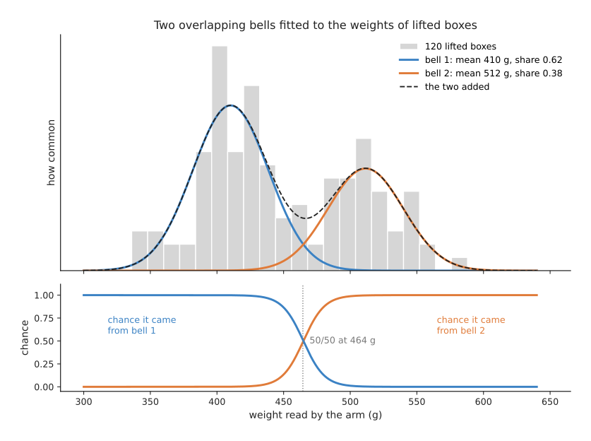
The fitted bells have means of 410 g and 512 g, both with an sd of about 28 g. Their shares are 0.62 and 0.38, close to the true 70 and 50 out of 120.
The lower panel shows the most useful output, because for any weight the model gives the chance that it came from each bell. A box of 440 g has a 0.04 chance of being full, while a box of 455 g has 0.23 and one of 470 g has 0.64. The two chances are equal at 464 g. This is a soft answer, because near the middle the model says "not sure" instead of forcing a yes or no.
Fitting the bells: expectation and maximisation#
The bells are fitted by a method called expectation–maximisation (EM), which solves a problem where each half needs the other half first. If we knew which box came from which bell, fitting each bell would be easy, because we could take the average and spread of its boxes. If we knew the bells, saying which box came from which would be easy, because we could compare the heights of the bells at that weight. We know neither, so EM guesses one and improves both in turn.
- Start with a guess for each bell, which is a mean, a width and a share, and the script started with means of 380 g and 560 g.
- Expectation step. For each reading, work out the chance that it came from each bell, using the current bells. This gives each reading a set of fractions that add up to 1, such as 0.9 for bell 1 and 0.1 for bell 2.
- Maximisation step. Then refit each bell from all the readings, but count each reading only by its fraction for that bell. So a reading that is 0.9 bell 1 counts almost fully towards bell 1, and hardly at all towards bell 2.
- Then repeat steps 2 and 3 until the bells stop moving.
For the box weights, EM stopped after 11 rounds of those two steps.
EM is k-means with soft edges. K-means, from Book 6's clustering page, gives each point wholly to its nearest centre, while EM gives each point partly to every bell. EM also learns each bell's width and tilt, which k-means does not.
A run in two dimensions#
The box weights were one number each, and in two dimensions each bell becomes an oval hill instead. Its covariance is a small table of numbers that says how wide the oval is in each direction and how it is tilted.
The next picture uses 200 points where a person dropped parts onto a tray, in three loose heaps, and EM starts from three large round guesses near the middle.
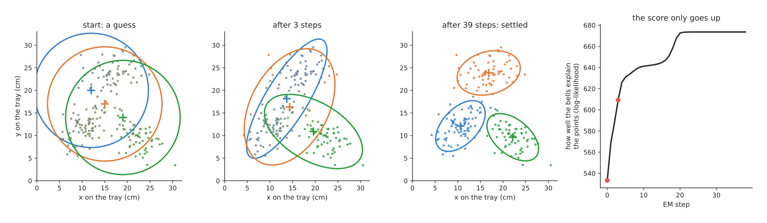
Each point is coloured by its fractions: a pure colour means one bell claims it, and a mixed colour means it is shared. The ovals show two sds around each mean. After 3 rounds the ovals have stretched towards the heaps, but two of them still share one heap. Then after 39 rounds they have settled. The fitted means are (10.6, 12.1), (16.8, 23.9) and (22.1, 9.6) centimetres, against true means of (10, 12), (17, 24) and (22, 10). The shares are 0.39, 0.31 and 0.30, against true shares of 0.40, 0.30 and 0.30.
The right panel shows the log-likelihood, which is a score for how well the bells explain the points, where higher is better. It rose from 533.3 to 673.6, and it never went down. That is always true of EM, so it is a useful check on your own code.
3. Gaussian mixture regression: a motion from a few demonstrations#
Section 2 used a mixture to say which source a reading came from, and Gaussian mixture regression (GMR) turns the same mixture into a way of predicting one number from another. On a robot arm it is used to learn a motion from a few demonstrations.
A demonstration is one recording of a person doing the motion. A common way to record one is hand-guiding, also called kinesthetic teaching: a person holds the arm and moves it through the motion, while the arm's joints and the position of its hand are recorded.
The script recorded five demonstrations of lifting a cup, carrying it and setting it down, and each one gives the cup's height at 60 moments. Time is written from 0 at the start to 1 at the end, so that fast and slow demonstrations line up.
- Put every recorded point from all five demonstrations into one table with two columns: time and height. That is 300 points.
- Then fit a mixture of five bells to this table with EM, so that each bell ends up covering one part of the motion: the lift, the top, the lowering, and so on. Each oval is tilted along the direction the height changes at that part.
- To move the arm, ask the mixture: "at time t, what height?" Each bell gives its own answer, which is a straight-line guess along its tilt, and the answers are then blended, weighted by how much each bell covers time t.
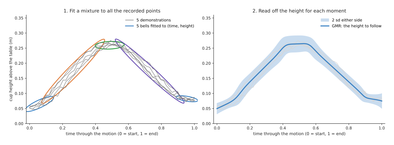
The blue curve is the height the arm follows, and it peaks at 26.5 centimetres (cm) about half-way through. GMR also gives a spread at every moment, shown as the pale band, and that spread is 8.9 millimetres (mm) at the start, 13.5 mm in the middle and 12.3 mm at the end. A controller can use it, because where the demonstrations agreed it can hold the path stiffly, and where they varied it can let the arm give way more.
GMR is more than an average, because the largest gap between the GMR curve and a plain average of the five demonstrations is 7.9 mm, since the demonstrations do not line up perfectly in time. The mixture smooths over that, so the result is one smooth curve with no corners.
The next page, movement primitives, covers two other ways to learn a motion from a few demonstrations, and they are used more often than GMR today, because they also adapt the motion to a new goal.
4. Hidden Markov models: states you cannot see#
Sections 2 and 3 treated every reading as independent of the last, but an HMM adds time. A hidden Markov model (HMM) tracks a situation that changes over time and that you cannot measure directly, so it works the situation out from readings that you can measure.
For example, a wiping tool comes down onto a table, presses, slides sideways, stops and slides again. The robot's program needs to know which of three states it is in: approaching, in contact or sliding. But no sensor reads the state, because the wrist sensor reads only the pressing force and the arm reads only the sideways speed, and both readings are noisy.
So the word hidden means that the state cannot be read. The word Markov, after the mathematician Andrey Markov, means the model assumes that the next state depends only on the current state, and not on the whole history.
The three parts of the model#
The wiping example needs all three parts of an HMM, which are these.
-
Starting chances. How likely each state is at the first reading, which here means that the tool almost always starts by approaching.
-
Transition chances. For each state, the chance of each next state one reading later. The table below shows them for the wiping tool, learned from a labelled recording taken at 50 readings a second. Read each row as "from this state"; the columns give the chance of each state one reading later.
From \ to approaching in contact sliding approaching 0.984 0.012 0.004 in contact 0.003 0.980 0.017 sliding 0.002 0.010 0.988 The large numbers on the diagonal say that the state usually stays the same from one reading to the next, and this is what lets the model ignore a single odd reading.
-
Reading chances. For each state, a bell over the readings. Approaching has a force near 0.0 newtons (N) and a speed near 0 mm per second, while in contact has 5.0 N and no speed, and sliding has 4.5 N and about 16 mm per second.
The forward algorithm: which state now?#
Those three parts describe the model, and the forward algorithm is how you use it live. The forward algorithm answers one question: given all the readings so far, what is the chance of each state now? It keeps one chance for each state, and it repeats two steps at every new reading.
- Predict. Move the chances one step on with the transition table. So if the tool was surely in contact, it is now in contact with chance 0.980 and sliding with chance 0.017.
- Update. Multiply each state's chance by how well the new reading fits that state's bell, then scale the three chances so they add up to 1.
These are the same two steps as the Kalman filter in Book 5. But the Kalman filter tracks a number, such as a position, while the forward algorithm tracks a choice between a few states. It uses only past readings, so it can run live on the robot.
Viterbi: the best whole story#
The forward algorithm looks only backwards, and the Viterbi algorithm looks at the whole recording instead. The Viterbi algorithm, named after Andrew Viterbi, answers a different question: after the whole recording, what single sequence of states best explains all of it? So it is used to split a recording into steps after the fact.
It works through the readings once, from start to end, and for each state at each reading it keeps only the best way of arriving there, with a note of which state that way came from. Then at the end it picks the best final state and follows the notes backwards. Because it looks at the whole recording, it can use a later reading to decide that an earlier moment belonged to one state rather than another.
A run on a force trace#
The script fitted the HMM from one labelled recording of 510 readings, and it then ran that model on a new recording of 310 readings, 6.2 seconds long, with 5 true changes of state.
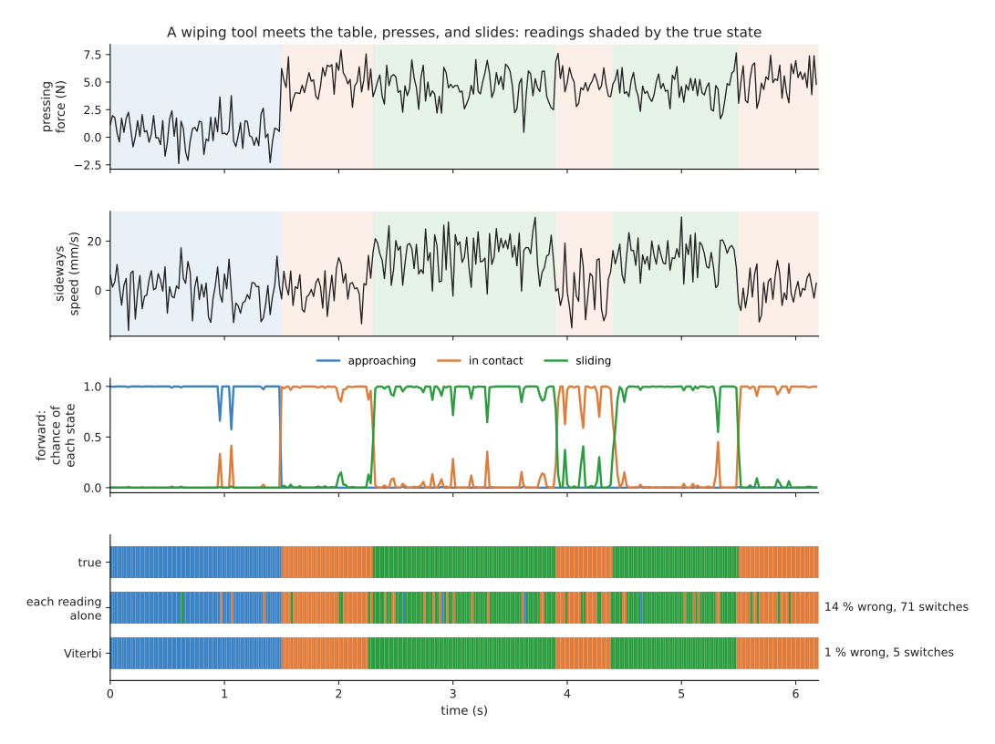
The top two panels show the readings, shaded by the true state, and the third panel shows the forward algorithm's chance of each state. The bottom panel then compares three answers.
The table below compares them. Read each row as one way of choosing the state.
| Method | Readings wrong | Changes of state reported |
|---|---|---|
| each reading alone, nearest bell | 13.9 % | 71 |
| forward algorithm, most likely state | 1.0 % | 5 |
| Viterbi, best whole sequence | 1.3 % | 5 |
Judging each reading alone flickers between states 71 times, because one noisy reading can look like any state. But both HMM methods report the true 5 changes. In this run Viterbi was very slightly worse per reading, because it chooses the best whole sequence rather than the best state at each moment. Both of them place every change within two readings, or 0.04 seconds, of the true moment. The forward algorithm is up to one reading late, because at each moment it has not yet seen the readings that follow.
5. How they are trained#
Sections 2 to 4 each fitted a model, so this section gathers what the fitting needs. A mixture needs only the readings, with no labels, but it does need you to choose the number of bells. A common way is to fit several numbers of bells and compare them with a score that punishes extra ones, such as the Bayesian information criterion (BIC). Tens of points per bell are usually enough in one or two dimensions, but many more are needed when each point has many numbers, because each bell's covariance has many entries to learn.
GMR needs a few demonstrations, typically 3 to 10, of the same motion, and each one must be lined up in time, usually by scaling each recording to run from 0 to 1.
An HMM can be trained in two ways. With a labelled recording, where someone has marked the state at each moment, training is just counting: count how often each state follows each other one, and fit a bell to each state's readings, which is what the script did. Without labels, a version of EM called the Baum–Welch algorithm learns all three parts from the readings alone. But it needs more data, and the states it finds may not match the ones you had in mind, so you usually give it a sensible starting guess.
6. Where they are used on a robot arm#
- Learning a motion from a few hand-guided demonstrations. GMR reproduces a smooth path with a spread, so a compliant controller can use that spread as a stiffness guide.
- Splitting a demonstration into steps. Viterbi splits a long recording of, say, a peg insertion into "reach", "align", "insert" and "release", so that each part can then be learned or checked on its own.
- Tracking contact. The forward algorithm follows the contact state live from force readings, so a program can switch its controller when the tool touches.
- Spotting that something went wrong. If a trained HMM or mixture gives a very low chance to the current readings, then the task is doing something it has never seen, which makes this a simple kind of failure detector.
- Sorting items by a measured number. A mixture sorts boxes, parts or grasps by weight, width or force, without anyone labelling them first.
- Describing where things usually are. A mixture over where objects were found on a table gives a map of the likely places to look first.
7. What goes wrong#
Section 5 said how these models are fitted, and this section says how the fitting fails. EM can settle on a poor answer, because where it ends depends on where it starts. Two bells can end up sharing one heap while another heap has none, as in the "after 3 steps" panel of the picture. So the fix is to start from k-means centres, or to run EM several times from different starts and keep the best score.
A bell can also shrink onto a single point, because its width goes to zero and its score goes to infinity. So the fix is to add a small number to every covariance at every step, and the script adds 0.000001.
The number of bells or states has to be chosen by you. With too few the model blurs different things together, while with too many it fits the noise. So compare scores such as BIC on held-back data.
A real state's readings may not follow a bell, because the force while sliding may have a long tail or two humps. So the fix is to use a mixture of bells for each state, or to feed the HMM better readings, such as a filtered force.
The Markov assumption is not quite true either. A real contact state lasts a typical time, but an HMM assumes the chance of leaving is the same at every reading, however long the state has lasted. For most contact tracking this does not matter, although for step splitting some people use a variant that learns how long each state lasts.
GMR only reproduces the demonstrated motion, because it does not know about a new goal or an obstacle. So movement primitives handle the new goal instead.
8. Libraries#
You would use a library rather than write EM and Viterbi yourself, so the table below lists the real ones. Read each row as one library and what it provides.
| Library | Language | What it provides | Note |
|---|---|---|---|
| scikit-learn | Python | GaussianMixture and BayesianGaussianMixture in sklearn.mixture | the place to start for mixtures; has bic for choosing the number of bells |
| hmmlearn | Python | GaussianHMM in hmmlearn.hmm, with fit, predict (Viterbi) and predict_proba | the standard small HMM library; follows the scikit-learn pattern |
| gmr | Python | a GMM class with a predict method for Gaussian mixture regression | small library by Alexander Fabisch, made for robot motions |
| pomegranate | Python | mixtures and HMMs, built on PyTorch | faster on large data; can run on a graphics card |
9. Why these, and what they cost#
The libraries make all three methods cheap to try, so this section says when to choose them. A Gaussian mixture describes data as a few overlapping bells, while an HMM tracks a hidden state from noisy readings over time, and GMR turns a mixture into a smooth motion.
What they do for you: they turn a handful of readings or demonstrations into a model that gives a chance for every answer, not just an answer. They also train in seconds, and you can look inside them, because each bell and each transition chance means something that you can check.
The obvious alternative to a mixture is k-means, and to an HMM it is a threshold on each reading. A mixture beats k-means when the groups overlap or have different widths, and when you want to know how sure the answer is. An HMM beats a threshold when the readings are noisy, because it uses the fact that states last, and the run above cut the error from 13.9 % to about 1 %. For learning a motion, the obvious alternative is a behaviour cloning network. GMR needs far fewer demonstrations and no camera, but it only learns one motion and cannot react to what it sees.
What they cost: you must choose the number of bells or states yourself, and EM can end in a poor answer, so it needs several starts. The model is also only as good as its bell shapes. And none of them read pictures, because the inputs must be a few meaningful numbers.
10. The written alternative#
Section 9 compared these methods with other learned ones, but Book 5 does all three of their jobs without learning. For sorting readings into groups, Book 6's clustering page does the same job with k-means or mean shift. It wins when the groups are well apart, while the mixture wins when they overlap.
For tracking contact, the written way is a threshold with a finite state machine: switch to "in contact" when the force stays above a set value for a few readings, as in the guarded moves of Book 5. It wins when the readings are clean and the states are few, because it is easy to read and to test. But the HMM wins when the readings are noisy, when several readings must be combined, or when you want a chance rather than a yes or no.
For reproducing a motion, the written way is to pick a few waypoints by hand and let trajectory generation join them smoothly. It wins when you can say where the path should go, while GMR wins when the motion is easier to show than to describe.
11. Where to read next#
- The next page is movement primitives, which learns a motion from demonstrations and then adapts it to a new goal.
- The chapter overview compares all the classical methods.
- Force and slip models covers neural networks that read force signals, for when an HMM is not enough.
- Behaviour cloning learns movement from many demonstrations with a network.
- Book 6's Kalman filter explains predict and update for a continuous number.
12. Using it in Python#
Section 2 fitted a mixture of bells with expectation and maximisation, section 4 found the best path through hidden states with Viterbi, and section 8 named the libraries. This section shows the calls, so that after reading it you can fit both models to recorded readings without writing either algorithm.
from sklearn.mixture import GaussianMixture
from hmmlearn import hmm

# X has one row per reading. covariance_type="full" lets each bell be tilted,
# and n_init=10 runs the fit from ten different starts and keeps the best.
mixture = GaussianMixture(
    n_components=3, covariance_type="full", n_init=10, random_state=0).fit(X)
print(mixture.bic(X))                  # lower is better; try several n_components
print(mixture.predict_proba(X_new))    # section 2's share for each bell

# forces holds three recorded traces stacked one after the other, and lengths
# says how many rows each trace has.
chain = hmm.GaussianHMM(n_components=3, covariance_type="diag", n_iter=100)
chain.fit(forces, lengths=[200, 180, 210])
print(chain.predict(new_trace))        # section 4's Viterbi path
print(chain.predict_proba(new_trace))  # section 4's forward probabilities
The lengths argument is the detail that catches people, and it is worth
understanding rather than copying. If you leave it out, hmmlearn treats the whole
array as one single long trace, so it learns a transition from the last state of
one recording to the first state of the next. Those transitions never happen on
the robot, and the model then reports state changes that are not there.
The libraries give you both of the algorithms this page worked through. The
expectation and maximisation loop of section 2 is inside GaussianMixture.fit,
and the Baum-Welch training of section 5 is inside GaussianHMM.fit. Viterbi is
predict and the forward algorithm is predict_proba, so the two algorithms
that section 4 spent most of its length on are one method call each. They also
handle two of section 7's failures for you: n_init above is section 7's advice
to run the fit from several starts, and GaussianMixture adds 0.000001 to every
covariance by default, through its reg_covar argument, which stops a bell
shrinking onto a single point. Section 8's gmr package adds the Gaussian
mixture regression of section 3, which scikit-learn does not provide.
What you have to collect is the recordings, and for the HMM you have to keep them
separate so that you can pass lengths. Section 3's mixture regression needs
several demonstrations of the same motion, resampled onto a common time axis,
which is preparation you do before any of this code runs.
What you have to decide is n_components, which is how many bells or how many
hidden states, and covariance_type, which is how much shape each bell is
allowed. bic above helps with the first, because you fit the model for several
values and keep the one with the lowest score, and section 7 said that this
number has to be chosen by you because too few bells blur different things
together and too many fit the noise. For covariance_type, "full" fits a
tilted bell and needs the most data, while "diag" assumes the columns vary
independently and needs much less, which is why the HMM above uses it.