This page explains decision trees, and the two ways of joining many trees together: random forests and gradient-boosted trees. It answers five questions, and the sections below take them in turn. How does one tree make a decision? How does it choose its questions? Why does a deep tree go wrong on new data? How do many trees fix that? And where does a robot arm use them?
It is for a reader who has read this book's first chapter, in particular how a model learns. So you need to know what an example, a label, a training set, a test set and overfitting are. The overview of this chapter shows where trees sit among the other classical methods.
Trees are the most used learned method for tabular data, which means data that fits in a table, where each row is one example and each column is one measured number. So on a robot arm that kind of data means logged grasps, force readings, motor currents and temperatures.
Every number on this page comes from a real run of the diagram script
docs/diagrams/classical_ml_2.py. The data is simulated from a made-up rule, so
that the true answer is known. But the methods themselves are real, and they are
written in NumPy.
Contents#
- The idea in one sentence
- How one tree works · Choosing a question · Depth, and overfitting
- Random forests: many trees vote
- Gradient-boosted trees: each tree fixes the last one's mistakes · Sample weights: the first way to boost · Fitting the remaining error · The learning rate
- Feature importance: which columns mattered
- How it is trained: what data, and how much
- Where it is used on a robot arm
- What goes wrong
- Libraries
- Why trees, and what they cost
- The written alternative
- Where to read next
- Using it in Python
1. The idea in one sentence#
A decision tree reaches an answer by asking a short chain of yes-or-no questions, each about one input number, and it learns which questions to ask, and in what order, from examples.
For example, a doctor on the phone decides whether you need to come in. "Is your temperature above 38 degrees? If yes, have you had it for more than three days?" Each question looks at one thing, and the answer to one question decides which question comes next. After two or three questions the doctor has an answer, and a decision tree works the same way. The difference is that nobody writes the questions, because the tree picks them itself by looking at many past cases.
A decision tree is not the same thing as a behaviour tree, which is a hand-written plan that decides what a robot does next. Book 5 explains those in behaviour trees, and the two kinds of tree share only the word "tree".
2. How one tree works#
Section 1 said that a tree learns its questions from examples, so this section follows one tree while it does that. The example on this page is a slip detector, where a robot gripper holds an object. A force sensor in each finger measures two forces, which are how hard the fingers squeeze and how hard the object pulls sideways along the finger pads. Then the program computes two features from those readings, where a feature is one input number, made from the raw readings, that the model uses.
- The sideways ratio is the sideways force divided by the squeezing force, and it runs from 0 to 1 here. When it gets near the friction of the surface, the object starts to slide.
- The shaking is how much the force signal shakes quickly, again from 0 to 1, and it matters because a slide makes the force shake before the object falls out.
Each example is one short moment of a grip, and its label says "slipping" or "holding". The made-up true rule is that the object slips when the ratio is above 0.62, or when the ratio is above 0.38 and the shaking is above 0.55. The script then flips 8% of the labels at random, because real labels are never perfect, and this makes the problem fair. So it has 200 examples to learn from, and 4,000 more to test on.
Choosing a question#
A tree grows from the top, so at the start all 200 examples sit in one group. The tree then looks for one question that splits that group into two groups that are as "pure" as possible, where a pure group holds only one label.
To measure how mixed a group is, trees usually use the Gini impurity, which for a group with a share p of "slipping" examples is 2 × p × (1 − p). It is 0 when the group is pure, and 0.5 when the group is half and half. The 200 examples hold 106 slipping and 94 holding, so the Gini impurity at the top is 0.498.
For a split into two groups, the tree takes the Gini impurity of each group, weights it by the group's size, and adds the two. Then it searches:
- Take the first feature, and sort the examples by it.
- Then try a cut between every pair of neighbouring values, and for each cut compute the weighted Gini impurity of the two groups.
- Do the same for every other feature in the table.
- Keep the cut with the lowest value, because that cut becomes the question at this point in the tree, which is called a node.
The picture below shows this search for the first question.
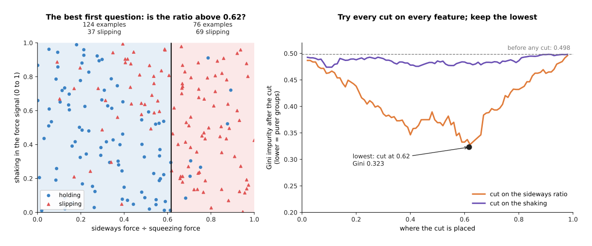
The right half shows the result of every possible cut. Cuts on the shaking barely help, because the best one, at 0.09, only brings the value down to 0.474. Cuts on the sideways ratio help much more, since a cut at 0.2 gives 0.438, a cut at 0.5 gives 0.369, and the lowest is at 0.617, which gives 0.323. So the first question is "Is the sideways ratio above 0.617?". The left group then holds 124 examples, 37 of them slipping, with a Gini impurity of 0.419, while the right group holds 76 examples, 69 of them slipping, with a Gini impurity of 0.167.
The tree then repeats the same search inside each group, and again inside each of their groups. Each group that is not split any further is called a leaf, and a leaf's answer is the most common label of the training examples in it. Its share of "slipping" examples can also serve as a rough chance.
The search is greedy, which means it picks the best question for this step only, without looking ahead. This is fast, but it can miss a pair of questions that would only help when they are used together.
Depth, and overfitting#
The search above never stops on its own, so the size of the tree has to be limited. The depth of a tree is the largest number of questions on any path from the top to a leaf, and if you let it, a tree keeps splitting until every leaf is pure. So the picture below compares a tree of depth 3 with a tree that has no limit.
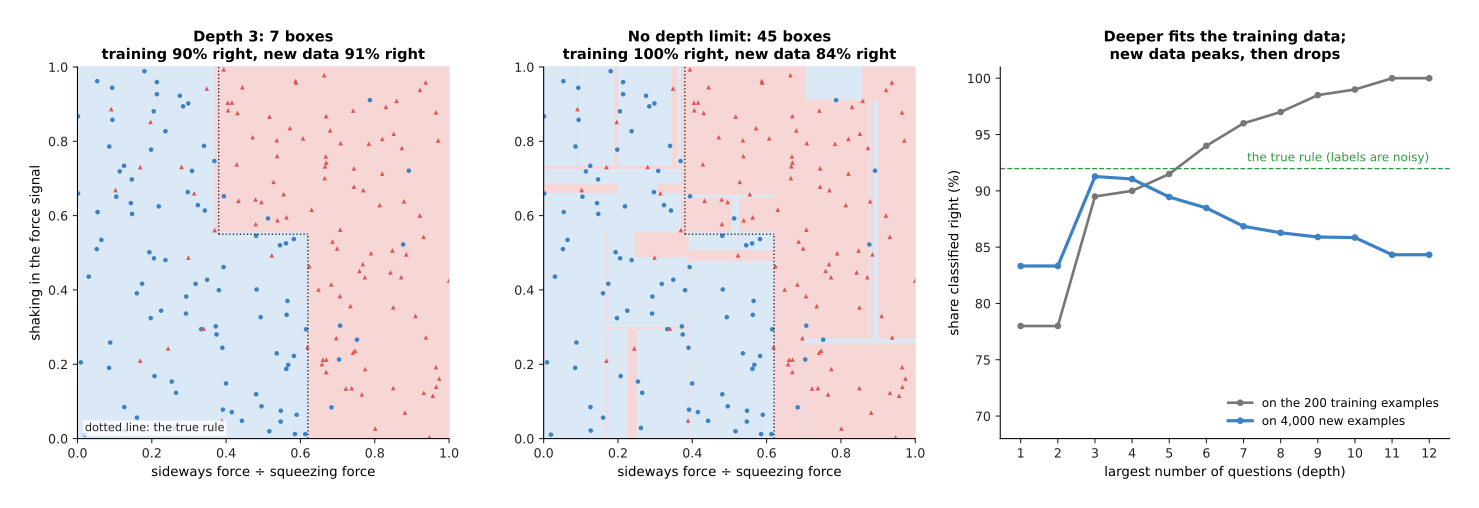
The tree of depth 3 found the questions below, and you should read them from the top.
- Is the sideways ratio at most 0.617?
- Yes: is the shaking at most 0.553?
- Yes: say "holding". (Its third question, on the ratio, only makes these groups a little purer.)
- No: is the ratio at most 0.369? If yes, say "holding". If no, say "slipping".
- No: say "slipping". (Its extra questions split off one single example near 0.684.)
- Yes: is the shaking at most 0.553?
This is close to the true rule, with cuts at 0.617, 0.553 and 0.369, against the true 0.62, 0.55 and 0.38. But the one-example box is the first sign of the problem that deeper trees have.
The tree with no limit grew to depth 11, with 45 leaves, and it gets every training example right. It does so by drawing thin boxes around each flipped label, so on new data it does worse, at 84% right against 91% for depth 3.
The right half of the picture shows the pattern behind those two numbers. Read the grey line as the score on the training examples and the blue line as the score on new examples, and the table below gives some of the same numbers.
| Depth | 1 | 2 | 3 | 4 | 6 | 8 | 11 |
|---|---|---|---|---|---|---|---|
| Right on the 200 training examples | 78.0% | 78.0% | 89.5% | 90.0% | 94.0% | 97.0% | 100% |
| Right on 4,000 new examples | 83.3% | 83.3% | 91.3% | 91.0% | 88.5% | 86.3% | 84.3% |
Two things stand out in that table. First, depth 2 is no better than depth 1, because its second question makes the groups purer without changing any group's answer. Only the third question changes an answer, and this is the greedy search at work. Second, the score on new data peaks at depth 3 and then falls, while the training score keeps rising, which is overfitting. The true rule itself only gets 92% of the new examples right, because 8% of the labels are flipped, so the depth-3 tree is almost as good as possible.
The usual limits are a largest depth, or a smallest number of examples per leaf, and the right setting is found by trying several of them on examples the tree did not train on. One tree is simple and easy to read, but it is also brittle, because a few different training examples can change its first question, and then everything below it changes too.
3. Random forests: many trees vote#
One tree is brittle, and a random forest answers that by growing many deep trees, each on a slightly different version of the data, and letting them vote. Its steps are:
- Draw a new training set of the same size from the original, by picking examples at random with replacement, so that some examples are picked twice or more and some are left out. This is called a bootstrap sample.
- Grow a tree on that sample, but at each node let the tree look at only a random few of the features rather than all of them, because this makes the trees differ more from each other.
- Then repeat both of those steps, for 100 to 500 trees in all.
- To answer a new case, ask every tree, and each tree gives one vote. The answer is the label with the most votes, and the share of votes serves as a rough chance.
Each tree is overfitted in its own way, because each one saw different examples. Their mistakes therefore point in different directions, so the vote cancels much of them out. But the parts they agree on are the parts that come from the true rule.
The script grew 200 trees, where each tree looks at one of the two features at each node and grows until its leaves hold 3 examples or fewer.
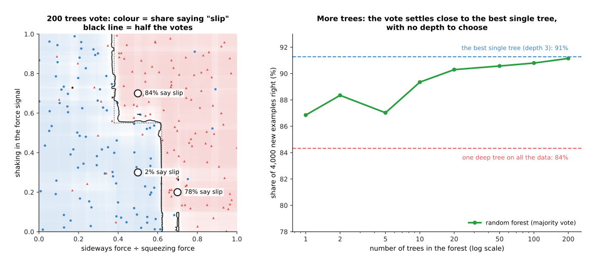
The left half colours each point of the plane by the share of trees that say "slip", and the black line is where half of them do. So that line follows the true rule, the dotted line, more smoothly than any single deep tree does. The three circles show some individual votes. At a ratio of 0.5 and shaking of 0.7, 84% of trees say slip, while at a ratio of 0.5 and shaking of 0.3 only 2% do. At a ratio of 0.7 and shaking of 0.2, 78% do, which is right but less sure, because a few flipped labels sit there.
The right half shows the score on new data against the number of trees. One tree from the forest gets 87% right, and the 200 single trees score 81% on average, with anything from 65% to 89%. Their vote gets 91.1% right, which is about as good as the best single tree at 91.3%, and nobody had to choose its depth. Adding more trees never makes a forest overfit more, because it only makes the vote steadier, at the cost of more time.
The vote is an equal vote, because every tree counts the same. The next method instead gives different trees different weights.
4. Gradient-boosted trees: each tree fixes the last one's mistakes#
A forest grows its trees side by side, each one on its own, but boosting grows them one after another instead. Each new tree looks at what the trees so far still get wrong, and it tries to fix that. The trees in boosting are small, often with a depth of 2 to 6.
Sample weights: the first way to boost#
The first boosting method, AdaBoost, short for "adaptive boosting", uses sample weights, where a sample weight is a number attached to each training example that says how much it counts. A tree that gets a heavy example wrong therefore pays more than one that gets a light example wrong. So the Gini search from section 2 simply counts weights instead of examples.
- Give every example the same weight, so that with 200 examples each weight is 1/200, or 0.005.
- Then grow a very small tree, often with only one question, and a tree with one question is called a stump.
- Measure its weighted error: the total weight of the examples it gets wrong.
- Give the stump a say, a number that is large when its error is small.
- Raise the weight of every example it got wrong, and lower the weight of every example it got right. Then scale all weights so they add up to 1.
- Then go back to step 2 and grow the next stump.
At the end every stump votes, and each vote counts as much as that stump's say, which is called a weighted vote.
On the slip data, the first stump asked "Is the ratio above 0.617?" and got 44 of 200 examples wrong, which is a weighted error of 0.22, so its say was 0.63. The weight of each example it got wrong then rose from 0.005 to 0.0114, while the weight of each example it got right fell from 0.005 to 0.0032. After this step the 44 wrong examples hold half the total weight, which always happens in AdaBoost. So the second stump cannot ignore them, and it chose a different question, "Is the ratio above 0.298?".
Sample weights are useful outside boosting too, because every library on this page lets you pass a weight per example when you train. For example, a robot project uses this to make rare failures count more, or to make recent data count more than old data.
Fitting the remaining error#
Gradient boosting is the method most used today, and it does the same job in a more general way. Instead of changing weights, each new tree learns the error that is left over.
The example here is predicting grasp success. Each row is one logged grasp, with six columns: the object's weight in kilograms, its width as a share of the gripper's opening, the grip force in newtons, the friction of the surface, the approach angle away from straight down in degrees, and the room temperature. The label is "held" or "dropped". The made-up true rule depends on the holding force compared with the weight, on objects near the gripper's full opening, and on steep approach angles, while the room temperature does not matter at all. The script has 600 grasps to learn from, of which 74% held, and 4,000 more to test on.
For a yes-or-no label the model keeps a running score for each example, and that score becomes a chance between 0 and 1 by the same squashing step that logistic regression uses. The steps are:
- Start every score at the same value: the one that gives the overall success rate, 74%.
- For each example, work out the gap between its label (1 for held, 0 for dropped) and its current chance.
- Grow a small tree that predicts those gaps from the six columns.
- Add a small share of that tree's answer to each score.
- Then go back to step 2 and grow the next tree.
The name of the method comes from step 2, because the gap is the gradient of the error measure, which is the direction in which the score should move. Chapter 1 explained gradients in how a model learns.
The learning rate#
The share in step 4 is the learning rate, and it decides how much of the error one tree may fix. With a learning rate of 1.0 each tree tries to fix all of the remaining error at once, while with 0.1 it fixes a tenth of it and leaves the rest to later trees.
To score the model, the script uses the log loss, which is an error measure for chances. A confident right answer costs almost nothing, while a confident wrong answer costs a lot, so a lower log loss is better. For example, a flat guess of 74% for every grasp scores 0.567, and the true chances, which no model can beat, score 0.302.
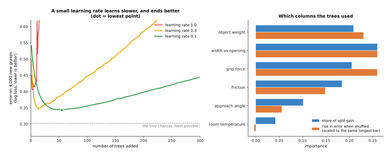
The left half shows the error on new grasps as trees are added, where each tree has a depth of 3. The table below gives the same results, and you should read each row as one learning rate.
| Learning rate | Lowest log loss | Reached after | Log loss after 300 trees |
|---|---|---|---|
| 1.0 | 0.407 | 3 trees | 1.359 |
| 0.3 | 0.348 | 13 trees | 0.739 |
| 0.1 | 0.343 | 55 trees | 0.444 |
A large learning rate learns fast and then overfits fast, so its best point is poor and it gets much worse with more trees. A small rate learns slowly, but it reaches a better best point and stays near it for longer. At its best the rate-0.1 model gets 84.8% of new grasps right, against 85.6% for the true chances.
Unlike a forest, boosting does overfit if you add too many trees. So people keep some examples aside, watch the error on them as trees are added, and stop when it stops falling. This is called early stopping, and a learning rate of 0.05 to 0.1 with early stopping is a common start.
5. Feature importance: which columns mattered#
Sections 3 and 4 both ended with hundreds of trees, which nobody can read, but a tree model can still tell you which columns it relied on. This is called feature importance, and there are two common ways to measure it.
The first way adds up how much each column's questions lowered the error, over every question in every tree, and this is called the split gain. It is free, because the trees computed it while they were growing.
The second way is permutation importance, which means taking the test examples, shuffling one column so that its values land on the wrong rows, and measuring how much worse the model gets. A column the model needs makes it much worse, while a column it does not need changes nothing.
The right half of the picture above shows both measures for the rate-0.1 model, and you should read each pair of bars as one column. The width as a share of the opening, the grip force and the object's weight matter most, because shuffling each of them raises the log loss by about 0.27 to 0.31. The friction matters a little less, and the approach angle less again.
The room temperature is the lesson here, because it had no effect in the true rule. Yet it got 4% of the split gain, since a tree can always find some cut on a noisy column that helps a little on the training data. Shuffling it did nothing at all, because the log loss changed by only −0.004. So the split gain can give credit to a useless column, and permutation importance on test data is the more honest check. Neither one says that a column causes success, because they say only what this model used.
6. How it is trained: what data, and how much#
Section 5 read the importance out of a trained model, and this section says what a model needs before you can train one. A tree model needs a table, where each row is one example and each column is one number that the robot can measure at the moment it must decide. The label is the answer you want, which can be slip or hold, success or failure, or a number.
Trees need little preparation of the data. Columns can have very different units, such as kilograms next to degrees, because each question looks at one column on its own, so you do not need to scale the columns. Some libraries also handle missing values and columns of categories, such as the kind of gripper.
How much data depends on how many columns and how complicated the true rule is. As a rough guide:
- A few hundred rows are enough for a useful model with 5 to 10 columns, as in this page's examples.
- Thousands of rows let boosted trees find finer patterns.
- With under about 100 rows, a single shallow tree or logistic regression is safer.
Training takes seconds on an ordinary computer for tables of this size. Keep separate test examples, and if the rows come from runs over time, test on a later run than you trained on. Otherwise you test on examples very like the ones the model has already seen, and the score looks better than it is.
7. Where it is used on a robot arm#
Section 6 said that trees want a table of measured numbers, and a robot arm logs exactly that, so trees turn up in five places on an arm. Classifying contact and slip from force features. This is this page's first example, where a window of force readings becomes a few numbers, such as the sideways ratio, the shaking, and how fast the force is changing. A small tree or forest then says "slip" or "hold" in well under a millisecond. The page force and slip models covers the problem, and the networks used when the input is a raw signal.
Predicting grasp success from simple features. A robot logs every grasp: the object's size and weight, the grip force, the approach angle, and whether it held. Boosted trees then learn which grasps tend to fail, so the robot can raise the force or pick another grasp before it tries.
Ranking candidate grasps. A grasp planner proposes several grasps, and the model gives each one a chance of success, so the robot tries the highest first. The script ranked six grasps on the same mug (0.35 kg, friction 0.5) with the rate-0.1 model from section 4, and the table below lists them in the model's order. Read each row across: what changes in that grasp, the model's chance, and the true chance from the made-up rule.
| Rank | The grasp | Model's chance | True chance |
|---|---|---|---|
| 1 | narrow grip (0.40 of the opening), 35 N, 15° | 0.98 | 1.00 |
| 2 | 0.55 of the opening, 25 N, 5° | 0.98 | 0.99 |
| 3 | 0.55 of the opening, 25 N, steep 40° | 0.94 | 0.97 |
| 4 | 0.55 of the opening, weak 12 N, 5° | 0.88 | 0.96 |
| 5 | 0.55 of the opening, very weak 6 N, 5° | 0.47 | 0.80 |
| 6 | near full opening (0.95), 25 N, 5° | 0.03 | 0.72 |
The order is exactly the true order. The chances at the bottom are too low, because few training grasps look like these ones, but for ranking it is the order that matters and not the chance itself. The page grasp quality models covers networks that score grasps straight from a picture.
Spotting faults in logs. Motor currents, temperatures and tracking errors, labelled with past faults, train a model that flags a joint going wrong. The page collision and failure detection covers this kind of detector.
Choosing between a few actions. From a few numbers about the scene, a tree can pick which of several hand-written grasp or push routines to run. A small tree can also be printed and read, so people can check which routine it will choose.
8. What goes wrong#
Section 7 listed where trees work well, and this section lists the ways they fail, because each problem below has a usual fix.
A single deep tree overfits, because it gets every training example right and new ones wrong, as section 2 showed. So the fix is a depth limit or a smallest leaf size, chosen on held-out data, or a forest instead of one tree.
Boosting overfits too, if you add too many trees, so the fix is a small learning rate with early stopping, as in section 4.
Trees cannot answer beyond their data, because each leaf gives an answer it saw in training. For a number to predict, a tree never goes above the largest label or below the smallest, so its prediction goes flat beyond the last example. So the fix is to collect data over the whole range the robot will meet, or to use a method that follows a trend, such as linear regression.
Trees draw boundaries as staircases. Each question cuts along one column, so a diagonal boundary, such as "slip when sideways force is more than half the squeezing force", becomes many small steps. So the fix is to give the tree the right feature, which here is the ratio, instead of the two raw forces. This means choosing good features matters more for trees than any setting does.
Rare labels get ignored, because if 2% of grasps fail, a model that always says "held" is already 98% right. So the fix is to give the rare examples larger sample weights, as in section 4, and to judge the model by how many failures it catches rather than by the share it gets right.
The chances are rough, because a forest's share of votes and a boosted model's chance are often too sure or not sure enough. So if the robot acts on the number itself, check it against real outcomes first, and the page uncertainty and confidence explains how.
Importance is misread, as section 5 showed when a useless column got credit. So use permutation importance on test data, and do not read it as cause and effect.
9. Libraries#
Nobody writes the Gini search of section 2 by hand in a real project, so the table below lists real libraries for trees. Read each row as one library: the classes it provides, and when to use it.
| Library | What it provides | When to use it |
|---|---|---|
| scikit-learn | DecisionTreeClassifier and DecisionTreeRegressor in sklearn.tree; RandomForestClassifier, AdaBoostClassifier, GradientBoostingClassifier and HistGradientBoostingClassifier in sklearn.ensemble; permutation_importance in sklearn.inspection | the place to start; one interface for every method on this page |
| XGBoost | xgboost.XGBClassifier and xgboost.XGBRegressor | fast, widely used boosted trees; can train on a graphics card |
| LightGBM | lightgbm.LGBMClassifier and lightgbm.LGBMRegressor | very fast on large tables |
| CatBoost | catboost.CatBoostClassifier | handles columns of categories with little preparation |
All of them take a sample_weight argument in fit, which is how you pass the
per-example weights of section 4. scikit-learn's export_text in sklearn.tree
prints a single tree as questions, much like the list in section 2. XGBoost and
LightGBM also have C interfaces, so a trained model can run inside a C++ robot
program.
10. Why trees, and what they cost#
Those libraries make trees cheap to try, so this section answers the four questions: what trees are, what they do for you, why them rather than the obvious alternative, and what they cost.
Trees are models that answer with a chain of one-column questions, and a forest or a boosted model adds up hundreds of those chains. So they turn a table of logged numbers into a yes-or-no answer, a chance or a predicted number, with little tuning and little preparation of the data.
The obvious alternative is a small neural network, since the rest of this book uses networks. But on a table of a few to a few dozen measured numbers, boosted trees usually match or beat a network. They need no scaling of the columns, they have fewer settings that matter, and they train in seconds without a graphics card. You can also read one small tree, or at least ask a forest which columns it used. A network wins when the input is raw, such as a picture, a point cloud or a long force signal, because trees need someone to turn those into a short list of meaningful numbers first.
The second alternative is logistic regression, which weights and adds the columns. It is simpler, it follows trends beyond the data, and its weights are easy to read. Trees win when columns matter only in some cases, for example when the approach angle matters only above 30 degrees, because a weighted sum cannot draw that without help.
What trees cost:
- They need good features, because it was the ratio, and not the two raw forces, that made this page's slip tree work.
- They cannot answer beyond the range of their training data.
- A forest or boosted model of hundreds of trees is no longer easy to read.
- Their chances need checking before the robot relies on the numbers.
- Boosting needs early stopping, and every tree model needs its settings checked on held-out data.
11. The written alternative#
Section 10 compared trees with other learned models, but the rules in Book 5 do the same jobs without learning at all. For slip, the rule comes from physics, because an object slides when the sideways force is more than the friction times the squeezing force. Book 6's sensor streams shows how to smooth the force readings, take how fast they change, and turn them into a flag with thresholds that do not flicker. For contact, the guarded moves in impedance and force control stop the arm when the measured force passes a set limit.
A hand-written rule is itself a tiny decision tree, so the difference between the two is only who writes the questions. The written rule wins when the physics is known and steady, for example with rigid objects of a known friction, because it needs no data and is easy to check. The learned tree wins when the thresholds depend on things you cannot measure well, such as wet or dusty surfaces, or when many columns interact. So a common middle way is to train a small tree, print it, and then check or adjust its questions by hand.
12. Where to read next#
- Linear and logistic regression is the simpler method to try first, and the source of the squashing step used in section 4.
- Gaussian processes and Bayesian optimisation gives an answer with an error bar, which trees do not.
- Nearest neighbours and locally weighted regression answers by looking up similar past examples.
- Support vector machines were the common classifier for small tables before trees took over.
- Force and slip models covers slip detection with networks on raw signals.
- Evaluation and failure explains how to test a model fairly before the robot relies on it.
13. Using it in Python#
Section 2 searched for the best question by hand, section 3 grew a forest of trees, and section 9 listed the libraries. This section shows what all of that looks like when a library does it, and the point of the section is how little code it is. A random forest, which section 3 described as hundreds of trees voting, is one line.
from sklearn.tree import DecisionTreeClassifier, export_text
from sklearn.ensemble import RandomForestClassifier, HistGradientBoostingClassifier

names = ["sideways_ratio", "shaking"]   # section 2's two features

tree = DecisionTreeClassifier(max_depth=3, random_state=0).fit(X, y)
print(export_text(tree, feature_names=names))   # prints section 2's questions

forest = RandomForestClassifier(n_estimators=300, random_state=0).fit(X, y)
print(forest.feature_importances_)              # section 5's importances
print(forest.predict_proba(X_new)[:, 1])        # the share of trees voting slip

boosted = HistGradientBoostingClassifier(
    learning_rate=0.1, early_stopping=True).fit(X, y)
The export_text line is worth running once, because it prints the tree as the
indented list of questions that section 2 showed, with your own column names in
it. That is the property section 10 called readability, and it is real only for a
shallow single tree, since 300 trees cannot be read.
The library gives you all of the arithmetic on this page. The Gini search of
section 2, the bootstrap sampling and the vote of section 3, and the residual
fitting of section 4 are all inside fit. early_stopping=True does section 4's
stopping for you, by holding some rows back and watching for the point where the
score on them stops improving, which is the check section 10 said every boosted
model needs. Every one of these classes also takes sample_weight in fit,
which is section 4's first way to boost.
What you have to collect is X and y, and what you have to build are the two
columns named above. Section 2 computed the sideways ratio by dividing the
sideways force by the squeezing force, and section 10 said that it was that
ratio, and not the two raw forces, that made the slip tree work. A tree chooses
among the columns you hand it and never combines two of them into a new one, so
that combining is your job and no setting of the library replaces it.
What you have to decide is max_depth, which section 2 tied directly to
overfitting, n_estimators, which is how many trees to grow, and
learning_rate for the boosted model, which section 4 explained. More trees in a
forest do not make it overfit and only cost time, so the depth and the learning
rate are the two settings actually worth searching over. You search them against
rows the model has not trained on, and section 6 added that when the rows come
from runs over time, those held-back rows should come from a later run.