Not every learned model on a robot is a neural network, because the older learning methods, often called classical machine learning, are still used every day next to neural networks. This chapter covers those older methods, and this first page is its overview, so it answers four questions. What is classical machine learning? Why does it still matter on robot arms in 2026? Which methods does this chapter cover, and which one fits which job? And when does a small dataset make one of them a better choice than a network?
It is for a reader who has read the first chapter of this book, especially what a model is and how a model learns. So you need to know what an example, a label, a weight, a test set and overfitting are before you start, because this chapter builds on all five of them. Nothing else about machine learning is assumed in this chapter.
Contents#
- What classical machine learning is
- Why it still matters on arms in 2026
- The pages in this chapter
- The methods side by side
- When a small dataset makes them the better choice
- How this chapter connects to the rest
- Where to read next
- Using it in Python
1. What classical machine learning is#
The name is the place to start, because it says what these methods are not as much as what they are. Classical machine learning means the learning methods that were worked out before neural networks took over, and that are not themselves neural networks. Most of them date from the 1950s to the 2000s. They are still learning methods, because each one turns examples into a model that makes predictions, and none of them is a rule that a person wrote by hand.
For example, a shop wants to guess how long a delivery will take from the distance it has to travel, and it has fifty past deliveries to learn from. Nobody would build a large neural network for fifty rows, so instead you would draw a line or a smooth curve through the fifty points and read the answer off it. In other words, classical machine learning fits a simple shape to a small table of numbers.
A neural network works differently, because it has many adjustable weights and can learn very complicated shapes, such as how pixels make up a mug. However, it needs many examples to set all those weights, and a lot of computing to train them. Instead, classical methods have far fewer settings, so they usually take a short list of numbers that already mean something, such as a distance, a force or a joint angle. These input numbers are called features, and because these methods work on features rather than on pixels, they do not read raw pictures well.
2. Why it still matters on arms in 2026#
Fitting a simple shape to a small table of numbers sounds like a weak tool next to a neural network. The rest of this book is indeed about neural networks, because large networks now do most of the seeing and much of the moving on robot arms. However, classical methods still matter beside them, and they matter for four reasons.
- Small data. Many jobs on an arm come with tens or hundreds of examples rather than millions, because each calibration run, each logged grasp and each demonstration costs robot time and a person's time. With so few examples a classical method usually learns as well as a network or better, and Section 5 shows this with real numbers.
- Error bars. Some classical methods, such as Gaussian processes, say how sure they are at every input with no extra work, so a robot can use that number to refuse an action, or to measure again, when the model is unsure.
- Speed. They train in seconds on an ordinary computer with no graphics card, and many of them predict in microseconds, which is fast enough for a control loop that runs a thousand times a second.
- Explainability. You can read a regression's weights or follow a small tree's questions, so when the arm does something wrong a person can see why, and a safety review can check the reasoning.
Because each family covers the other's weakness, classical and neural methods are also often used together. For example, a pretrained network turns a picture into a short list of numbers, and a classical method then learns the robot's own job on top of those numbers.
3. The pages in this chapter#
Because those four reasons do not all apply to every method, the chapter sorts its eight pages into two groups after this overview.
The most used group holds four general tools, and each one of them learns from a table of numbers. Because they are so general, each can be used for almost any job where the input is a few measured numbers, and they are the ones a robot arm project reaches for first:
- Linear and logistic regression. A weighted sum of features that predicts either a number or the chance of a yes, and the page also covers ridge regression and weighted least squares.
- Decision trees and forests. Chains of yes-or-no questions, grown either one tree at a time or many trees together, which is where gradient-boosted trees belong.
- Gaussian processes and Bayesian optimisation. A smooth curve with an error bar at every point, and a way to use those error bars to tune settings in a few tries.
- Nearest neighbours and locally weighted regression. These methods keep every example they were given, so they predict from the stored ones that are most like the new input.
The also used group holds methods with a narrower job. Two of them are built for motions and sequences over time, which is why they are common in robot learning from demonstrations. Another one is a helper that makes the data smaller before a second method uses it. The last one was once the leading method for classification, and it is used less now because trees and networks usually do better:
- Mixture models and hidden Markov models. Data described as a few overlapping blobs, a motion learned from those blobs, and a task split into hidden phases.
- Movement primitives. A motion learned from one or a few demonstrations that can be stretched to a new start and goal.
- PCA and shrinking data. Turning many numbers into a few that keep most of the information.
- Support vector machines. A dividing line between two classes, placed as far as possible from both.
So read the four most-used pages first, and read them in order, because they are the ones a project reaches for first. The also-used pages can then be read in any order, whenever your own task needs them.
4. The methods side by side#
Section 3 listed the pages in reading order, and the table below puts the same methods side by side so that you can pick one for a job you already have. Read each row across: the method, what it predicts, the data it needs, one place it is used on a robot arm, and the page that explains it.
| Method | What it predicts | Data it needs | An arm example | Page |
|---|---|---|---|---|
| Linear and ridge regression | a number | tens of rows; features chosen by hand | turning a force sensor's raw counts into newtons | regression |
| Logistic regression | the chance of a yes | tens to hundreds of labelled rows | the chance a grasp holds, from grip force and object width | regression |
| Decision trees, random forests, gradient-boosted trees | a number or a class | hundreds to thousands of rows; columns in any units | which logged grasps tend to fail; spotting a faulty joint from motor logs | trees |
| Gaussian process | a number with an error bar | tens to a few thousand rows | correcting a depth camera's error, and knowing where the correction is unsure | Gaussian processes |
| Bayesian optimisation | the next setting to try | one score per try; 20 to 50 tries | tuning a controller's gains or a grip force on the real arm | Gaussian processes |
| k-nearest neighbours, locally weighted regression | a number or a class, from similar stored examples | every example kept; few input numbers | reusing the grasp that worked on the most similar stored object | neighbours |
| Gaussian mixture model and regression, hidden Markov model | groups, a motion, or the current phase of a task | a few demonstrations or recordings | telling whether an insertion is in its approach, contact or push phase | mixture models |
| Movement primitives | a whole motion, adapted to a new goal | one to ten demonstrations | a pouring or wiping motion moved to a new cup or table position | movement primitives |
| Principal component analysis | a few numbers that stand for many | unlabelled rows | shrinking a hand's many joint angles to two or three that matter | PCA |
| Support vector machine | a class | tens to thousands of labelled rows | telling contact from no contact in a force signal | support vector machines |
Every method in the table takes a short list of meaningful numbers as input, or a short recording of such numbers. None of them reads a raw picture well, so raw pictures are left to the neural network chapters.
5. When a small dataset makes them the better choice#
The first of the four reasons in Section 2 was small data, and this test shows
that point with real numbers. It comes from the diagram script
docs/diagrams/what_models_are_3.py, and the data is simulated so that the true
answer is known and every error can be measured against it.
A robot arm has a depth camera, which is a camera that also measures how far away each pixel is. Its readings are a little wrong, and the error changes with distance, so to correct it the robot measures a flat board at known distances from 0.3 to 1.5 metres. Each measurement is one example, where the input is the distance and the label is the error of the reading in millimetres (mm), with about 1 mm of random noise.
The script trained four classical methods and a small neural network on this problem, with more and more examples each time. The network had one hidden layer of 64 neurons and was trained by gradient descent. For each number of examples, every method was trained 8 times on fresh random examples, so that one lucky draw of the data could not decide the result. Then each run was scored by the root mean square error (RMSE) against the true curve, which means squaring each difference, taking the average and then taking the square root. This is a typical size of the error in millimetres, so a lower number is better.
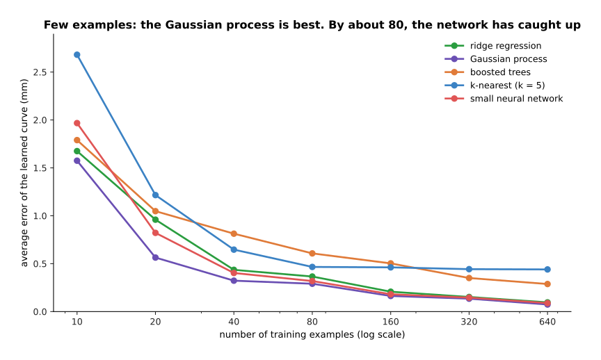
The table below gives the same results as the picture. Read each column as one number of training examples, and read each figure in it as the average error in millimetres.
| Method | 10 | 20 | 40 | 80 | 160 | 320 | 640 |
|---|---|---|---|---|---|---|---|
| Ridge regression | 1.67 | 0.96 | 0.44 | 0.37 | 0.21 | 0.15 | 0.10 |
| Gaussian process | 1.57 | 0.56 | 0.32 | 0.29 | 0.16 | 0.13 | 0.07 |
| Boosted trees | 1.79 | 1.05 | 0.81 | 0.61 | 0.50 | 0.35 | 0.29 |
| k-nearest (k = 5) | 2.68 | 1.22 | 0.65 | 0.47 | 0.46 | 0.44 | 0.44 |
| Small neural network | 1.97 | 0.82 | 0.40 | 0.32 | 0.18 | 0.15 | 0.09 |
Four things stand out in these numbers, and together they say when the extra power of a network is worth its cost.
- With 10 examples, the network is worse than the Gaussian process, ridge regression and the boosted trees.
- With 20 examples, the Gaussian process is clearly the best, at 0.56 mm against the network's 0.82 mm.
- By about 80 examples the network has caught up with the Gaussian process and ridge regression, and from there on the three stay close to each other.
- On this problem the network never pulls ahead, because the input is one number and the curve is smooth, so a network's extra power has nothing to do.
A network pulls ahead when the input is large and complicated, such as a picture or a long recording, and there are many examples to learn from. In that case no simple shape can describe the answer, so only a network can learn one, which gives the rule of thumb below:
- With a few numbers in and tens to hundreds of examples, try ridge regression, a Gaussian process or boosted trees first.
- With a picture, a point cloud or a sound in, and thousands of examples or more, use a neural network, usually one that someone else has already trained, as in fine-tuning.
- With both, a common mix is a network that turns a picture into a short list of numbers, and a classical method on top of those numbers.
6. How this chapter connects to the rest#
This chapter is not a separate world, since its methods connect backwards to Book 5 and forwards to the neural network chapters of this book.
Many classical methods share their maths with a written technique in Book 5, so the difference between the two books is the purpose rather than the formula. This means Book 5 fits a formula it already knows, while this chapter learns a shape that nobody wrote down. Linear regression is least-squares fitting used to predict. k-nearest neighbours is built on nearest-neighbour search. A Gaussian mixture model is a softer form of the k-means method in clustering. A hidden Markov model tracks a hidden state over time, as the Kalman filter does, but for a state that jumps between a few phases. Movement primitives are learned versions of the curves in trajectory generation. And Bayesian optimisation is a careful relative of sampling-based optimisation, built for when each try is expensive. So each method page in this chapter names its written alternative in Book 5.
To the neural network chapters. The later chapters of this book are about neural networks, and they meet the methods of this chapter in several places. Movement models learn from demonstrations, as movement primitives do, but from camera pictures and many more demonstrations. Grasp quality models score grasps with a network, where a logistic regression or boosted trees would score them from a few numbers. Learned arm models describes the Gaussian-process and locally weighted work on learning how an arm moves, which came before deep networks. Learned dynamics models often use a small classical model to correct a physics formula. And uncertainty and confidence explains how a robot uses an error bar, like a Gaussian process's, to decide whether to act.
7. Where to read next#
- The first page of this chapter is linear and logistic regression, and every other method in the chapter is easier once you know it.
- The map of models shows where this chapter sits among all the chapters of the book.
- Uncertainty and confidence explains how a robot turns an error bar into a decision.
- Fine-tuning covers adapting a pretrained network, including training a small classical model on top of it.
- Least-squares fitting in Book 5 explains the maths under linear regression.
8. Using it in Python#
Section 4 put the methods of this chapter side by side, and section 5 said that a small dataset is what makes them the right choice. This section adds the part those tables leave out, which is how much code any of them takes. The answer is four lines, and knowing that changes where you expect to spend your time.
from sklearn.ensemble import RandomForestClassifier
from sklearn.model_selection import train_test_split
from sklearn.metrics import accuracy_score

X_train, X_test, y_train, y_test = train_test_split(
    X, y, test_size=0.25, random_state=0)
model = RandomForestClassifier(n_estimators=300, random_state=0).fit(X_train, y_train)
print(accuracy_score(y_test, model.predict(X_test)))
Here X is a table with one row per example and one column per measured number,
and y is the answer for each row. Every method in this chapter follows the same
three calls, which are fit to learn from the training rows, predict to answer
for new rows, and a scoring function to say how well it did. So to try a support
vector machine instead you change RandomForestClassifier to SVC and nothing
else moves. That one property is why this chapter is worth reading before the
neural network chapters, because you can try five methods in an afternoon.
The library gives you the whole algorithm and a set of defaults that are usually
reasonable. It also gives you the splitting, the scoring, and Pipeline, which
chains a preparation step and a model together so that new data is prepared in
exactly the same way as the training data.
What you have to collect is X and y, and what you have to build is the
columns of X. That building is the real work of classical machine learning, and
this chapter calls those columns features. A feature is one number you
compute from the raw readings because you believe it carries the signal, such as
the ratio of sideways force to grip force rather than the two forces on their
own. Neural networks find their own features from raw input, and classical
methods do not, which is the trade section 1 described.
What you have to decide is which method to try, the handful of settings it takes, and how the split is made. Section 4's table is the guide to the first of those. For the third, remember that frames recorded a few milliseconds apart are nearly identical, so for data logged from a moving arm you split by run rather than by row, as where the data comes from explains.