This page explains two methods that belong together. A Gaussian process learns a smooth curve from a few examples, and it gives an error bar with every answer. Bayesian optimisation then uses a Gaussian process to decide which setting to try next, when every try is slow or costly, such as a test run on a real arm.
It answers five questions, and the sections below take them in turn. What does a Gaussian process predict, and how? What decides how smooth its curve is, and how much it trusts each measurement? Why does it get slow with many examples? How does Bayesian optimisation choose the next trial? And where does a robot arm use the two, for example to tune a controller in 15 trials instead of 100?
It is for a reader who has read the first chapter of this book, especially how a model learns. So you need to know what an example, a label and overfitting are. The chapter overview compares a Gaussian process with the other methods on one small dataset.
Every number on this page comes from a real run of the diagram script
docs/diagrams/classical_ml_3.py. The data is simulated, so that the true
answer is known exactly. But the methods themselves are real, and they are
written in NumPy.
Before this page, it helps to have read PID control in Book 5. The Bayesian optimisation examples tune its gains, on the same simulated joint.
Contents#
- The idea in one sentence
- How a Gaussian process works · The kernel: how alike are two inputs · Noise: how much to trust each measurement · A worked example: a correction to the friction model · Why it slows down with many points
- Bayesian optimisation: choosing the next trial · Tuning one gain, step by step · Two ways to choose: expected improvement and upper confidence bound · Tuning two gains in 15 trials
- How it is trained, and how much data it needs
- Where it is used on a robot arm
- What goes wrong
- Libraries
- Why this, and what it costs
- The written alternative
- Where to read next
- Using it in Python
1. The idea in one sentence#
A Gaussian process predicts a number together with an error bar, by assuming that similar inputs give similar answers, and Bayesian optimisation uses those error bars to pick each next trial where the answer looks good or is still unknown.
For example, you are adjusting a shower with a single knob. You try the middle and the water is too cold, then you try far to the right and it is too hot. You do not now try every position from left to right, because you can guess that the right temperature lies between your two tries, closer to the hot one, and you try there next. You also know how sure you are, since you are very sure near the positions you tried and less sure in between. A Gaussian process is that guess with its sureness written as numbers, and Bayesian optimisation is the habit of picking the next knob position from that guess.
2. How a Gaussian process works#
Section 1 called the shower guess a number with a sureness attached, so this section says what those two numbers really are. A Gaussian process (GP) takes a set of examples, which are inputs with a measured label for each. For any new input it gives two numbers, where the first is its best guess of the label. The second is a standard deviation, which is a typical size of how wrong that guess may be. This page draws the error bar as two standard deviations each side of the guess, so if the model is right about itself, the truth falls inside that band about 95 times in 100.
The name comes from the Gaussian, or normal, distribution, which is the bell-shaped spread of values. A GP treats the unknown curve as a random curve whose values are spread in that bell shape. It then keeps only the curves that pass close to the examples. So their average is the guess, and how much they disagree is the error bar.
You do not need to follow the maths to use a GP, because you only need to know the two things that you choose: the kernel and the noise.
The kernel: how alike are two inputs#
The kernel is a formula that says how alike the answers at two inputs should be, given how far apart the inputs are. So it gives 1 for two identical inputs, and falls towards 0 as the inputs move apart. The most used kernel falls in a bell shape, and it has two settings:
- the length scale: how far apart two inputs can be and still have similar answers;
- the signal size: how far the curve typically moves away from its average.
The left panel below shows this kernel with three length scales. With a length scale of 0.3, two inputs 0.1 apart score 0.95, which means nearly the same answer, while two inputs 0.3 apart score 0.61. Two inputs 1.0 apart score 0.00, so knowing one of them tells you nothing about the other.
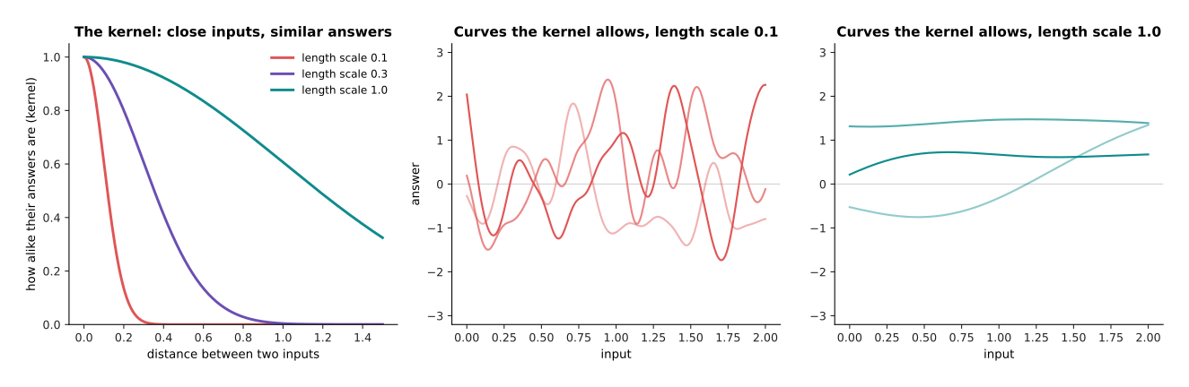
The two right panels show what the length scale means for the curve, because each panel draws three random curves that the kernel allows, before the GP has seen any example. A length scale of 0.1 allows curves that wiggle quickly, while a length scale of 1.0 allows only slow, gentle curves. So choosing the kernel is choosing what kind of curve you expect.
Then, to predict at a new input, the GP scores how alike that input is to each example, using the kernel. It then takes a weighted average of the examples' labels, with the more alike examples counting more. The error bar comes from those same scores, so if no example scores highly, the guess rests on little and the band is wide.
Noise: how much to trust each measurement#
A real measurement is never exact, so the GP has a third setting, the noise, which is the typical size of the error in each measured label. If the noise is small, the GP believes each example and bends its curve to pass through all of them. But if the noise is larger, it lets the curve pass between examples that disagree.
You rarely set these three numbers by hand, because the usual way is to try many combinations and keep the one under which the measured examples are most likely. This measure is called the marginal likelihood, and it prefers a curve that fits the examples while also punishing a curve that is more wiggly than the examples need. So it guards against overfitting by itself, without a separate test set.
A worked example: a correction to the friction model#
Book 5's PID page uses a joint whose friction follows a simple rule: 0.5 N m of torque for each radian per second of speed. But a real joint also has friction that this rule misses, and that extra friction is strongest just after the joint starts to move and changes sign with the direction. So the robot measures the missing torque at 24 speeds and wants a curve through them. The input is the joint speed in radians per second (rad/s), and the label is the missing torque in newton metres (N m). Each measurement has noise of 0.04 N m.
The measurements cover speeds from −1.0 to 0.45 rad/s, and a few more between 1.15 and 1.4 rad/s. So there is a gap between the two groups, and nothing beyond them.
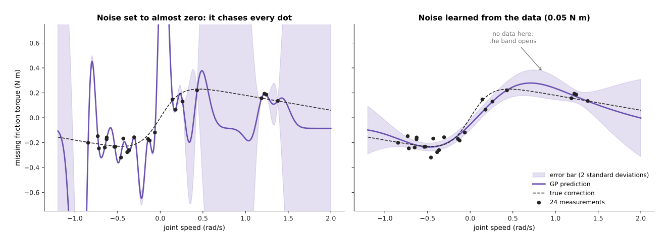
The left panel forces the noise to 0.001 N m, which is far below the true 0.04, so the GP must pass through every dot. To do that it chose a short length scale of 0.1 rad/s, and the curve swings wildly between the dots. Its average error against the true curve, over the measured range, is 0.804 N m, which is twenty times the noise.
But the right panel lets the marginal likelihood choose all three settings. It chose a length scale of 0.6 rad/s, a signal size of 0.2 N m and a noise of 0.05 N m, close to the true 0.04. So the average error over the measured range is 0.042 N m.
The table below reads the right-hand GP at four speeds, and each row gives the speed, where it lies, the GP's answer with its error bar, and the truth.
| Speed | Where it is | GP answer | True value |
|---|---|---|---|
| 0.0 rad/s | among the examples | −0.054 ± 0.042 N m | 0.000 N m |
| 0.8 rad/s | in the gap | 0.273 ± 0.108 N m | 0.203 N m |
| 1.3 rad/s | among the examples | 0.154 ± 0.053 N m | 0.144 N m |
| 1.9 rad/s | beyond all examples | 0.015 ± 0.278 N m | 0.072 N m |
So the band is narrow among the examples and wide in the gap and beyond. At 1.9 rad/s the GP says, in effect, "I do not know", because its band covers −0.26 to 0.29 N m. A controller can use that, since it can add the learned torque only where the band is narrow.
The first row shows a real weakness, because at 0.0 rad/s the truth lies just outside the band. The true friction changes sharply near zero speed, but the GP chose one length scale for the whole curve. A length scale of 0.6 is right for the gentle parts and too long for the sharp part, so the band is too confident exactly where the curve bends fastest. Section 6 returns to this.
Why it slows down with many points#
A GP keeps every example, and it compares each example with every other one, so the cost grows quickly with the number of examples. With n examples it builds a table of n × n kernel scores and solves a set of equations with it. The work to solve that grows with the cube of n, at about n³ / 3 multiply-adds. The script prints the numbers:
- 1,000 examples: about 3.3 × 10⁸ multiply-adds, which is a fraction of a second on a laptop, and the table takes 8 megabytes (MB).
- 10,000 examples: about 3.3 × 10¹¹, which is a thousand times the work, and the table takes 800 MB.
- 100,000 examples: a million times the work of 1,000, and a table of 80,000 MB, more memory than most computers have.
So a plain GP suits hundreds to a few thousand examples, which is often all a robot has, because each example is a real measurement. For more than that, libraries use approximations. The most common one keeps a few hundred inducing points, which are a small set of stand-in examples, and compares everything with those instead.
3. Bayesian optimisation: choosing the next trial#
Section 2 built a curve with an error bar, and Bayesian optimisation is what you do with that error bar when each try is slow or costly. It keeps a GP of the score against the setting, and it uses the GP's guess and error bar to pick the next setting to try. Then it runs the trial, adds the result to the GP, and repeats.
On a robot, a "try" is often a real run of the arm: a step move to test controller gains, or ten grasps to test an approach. Because each run takes seconds to minutes and wears the hardware, the aim is to find good settings in tens of trials rather than thousands.
Tuning one gain, step by step#
Here the joint from Book 5's PID page is told to move from 0 to 0.5 radians. The proportional gain Kp is fixed at 20, and the integral gain Ki at 5. So the task is to find the best derivative gain Kd between 0 and 2. The PID page explains the three gains.
Each trial runs the move for one second and gives one score, where lower is better. The score adds three things: the average distance from the target, how far the joint overshot the target, and how much the motor torque jittered from one tick to the next. Too little Kd overshoots, while too much Kd makes the torque jitter, because Kd multiplies the noise in the angle sensor. Each trial also has a little chance in it, because the sensor noise differs and the load changes by a few percent from run to run, as it does on a real arm.
A sweep of 201 settings shows the answer that the method does not know: the best Kd is 0.69, with a score of 11.02. But Kd = 0 scores 24.09, and Kd = 2 scores 21.85.
The loop that finds a setting like that works as follows.
- Run a few trials spread over the range, which here are Kd = 0.10, 1.00 and 1.90.
- Then fit a GP to the scores you have so far.
- For every Kd in the range, work out how promising a trial there would be. This number is called the acquisition function.
- Run the next trial where the acquisition is largest.
- Go back to step 2, until the trial budget is spent.
- Then keep the best setting that the loop found.
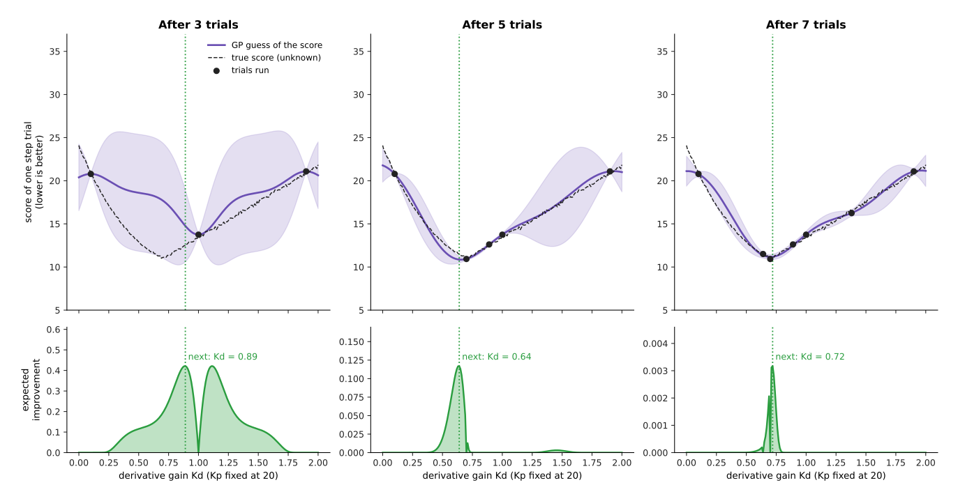
The top row shows the GP after 3, 5 and 7 trials. The bottom row shows the acquisition, and the dotted line marks the next trial.
- After 3 trials, the best score so far is 13.75, at Kd = 1.00. The GP knows little between the trials, so the band is wide and the acquisition is high on both sides of Kd = 1.00. It picks Kd = 0.89.
- The fourth trial, at 0.89, scores 12.62, so the GP now leans left and picks 0.70, and that trial scores 10.93.
- After 5 trials the GP has found the dip, so it picks 0.64, just beside the best.
- After 6 trials it picks 1.38, because that area was still unsure and the GP checks that nothing better hides there.
- After 7 trials it picks 0.72. After 8 trials, the best measured score is 10.77, at Kd = 0.72.
So eight trials found a Kd within 0.03 of the best one on a 201-point sweep. The best measured score, 10.77, is even lower than the swept best of 11.02, but that is not a better gain. It is one lucky trial, because the chance in each run happened to help. This is why the GP has a noise setting, and why a careful user re-runs the kept setting a few times before trusting its score.
Two ways to choose: expected improvement and upper confidence bound#
Step 3 of that loop left the acquisition function undefined, so this section fills it in. The acquisition function turns the GP's guess and error bar into one number per setting, and two of them are used most.
Expected improvement (EI) asks: if I try here, by how much will I beat my best score so far, on average? A setting scores high if the guess is already better than the best so far. It also scores high if the band is wide, because a wide band leaves room for a much better result. A setting whose whole band is worse than the best so far scores almost zero. This is why the bottom row above is zero at both ends, since the GP is sure those ends are worse.
Upper confidence bound (UCB) asks a simpler question: how good could it be here, if I am optimistic? So it takes the guess and moves it by a set number of error bars in the good direction. The name comes from problems where a higher score is better, so for a score where lower is better, as here, it is the guess minus the error bar. A setting wins if it looks good, or if it is so unsure that it might be good. The number of error bars sets the balance, because more error bars send trials to unexplored places, while fewer send them close to the best so far.
The balance between the two aims has a name: exploration, trying where the model is unsure, against exploitation, trying where the model is already hopeful. Both acquisition functions weigh those two aims, and in the one-gain run they agreed closely. After 3 trials expected improvement picked Kd = 0.89, while the bound with two error bars picked 0.83.
Tuning two gains in 15 trials#
Most controllers have more than one gain, so here Kp and Kd are tuned together. Kp may lie between 2 and 200, and Kd between 0.02 and 5. Both are searched on a log scale, where each step multiplies the gain by the same factor. People often do not know a gain's size to within a factor of ten, so a log scale spreads the trials fairly.
A sweep of 1,681 settings shows the landscape, where the best is Kp = 14.2 and Kd = 0.42, with a score of 10.83. Only 3.2% of the settings score within 1 of that, and the worst scores 76.1.
The script ran three methods, each with 15 trials, 20 times over with different chance. Both Bayesian optimisation runs start with 4 random trials and then let the GP choose the other 11, and the UCB run uses one error bar. The third method runs all 15 trials at random settings.
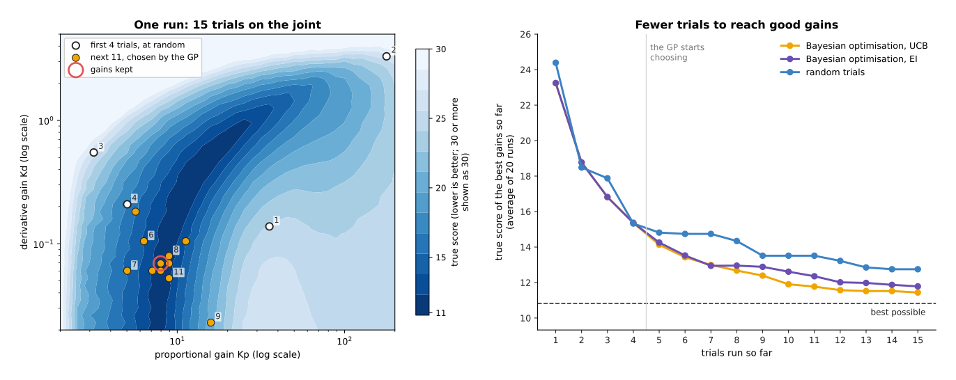
The left panel shows a typical run, which is the one whose result is the middle of the 20, and darker blue is a better score. The first 4 trials, at random, land in poor places, but from trial 5 on the GP moves into the dark valley and stays there. So it keeps Kp = 8.0 and Kd = 0.07, whose true score is 11.39. That is not the sweep's best setting, but the valley is long, and settings along it score nearly the same.
The right panel shows the average over 20 runs, where the score shown is the true score of the gains each method would keep at that point. The table below gives the result after all 15 trials, and you should read it across: the method, its average, and its worst of the 20 runs. The best possible is 10.83.
| Method | Average after 15 trials | Worst of 20 runs |
|---|---|---|
| Bayesian optimisation, UCB | 11.44 | 12.40 |
| Bayesian optimisation, EI | 11.78 | 18.22 |
| Random trials | 12.75 | 15.92 |
Bayesian optimisation with UCB reached 12.67 after 8 trials, while random trials needed all 15 to reach 12.75. So on this problem it saved about half the trials, and on a real arm, where each trial takes a minute and a person must watch, that matters.
Expected improvement did well on average, but one of its 20 runs ended at 18.22, because that run never found the valley in its 15 trials. No acquisition function is best on every problem, and with 15 trials one unlucky run can happen. So a common fix is to run the kept setting a few more times, and to compare it with the hand-tuned gains before accepting it.
4. How it is trained, and how much data it needs#
Section 3 spent its examples one trial at a time, so this section says how many a GP needs in general. A GP needs a table of examples, where an input may be several numbers and each input has one measured label. Training means choosing the kernel's settings and the noise, by the marginal likelihood, and after that the examples themselves are the model. Adding an example means refitting, which is quick while the examples number in the hundreds.
A GP works well from very few examples, because the friction curve above used 24 and the one-gain tuning used 8. So with 2 to 5 inputs, a few tens of examples often give a useful curve. The chapter overview showed a GP beating a small neural network with 10 and 20 examples.
It works less well with many inputs, because each input needs its own length scale and the space to fill grows fast. So Bayesian optimisation is usually used with up to about 10 or 20 settings, since beyond that the GP cannot learn the landscape from a few tens of trials.
Before fitting, scale each input to a similar range, for example 0 to 1, and subtract the average from the labels. In the two-gain example, the script also takes the logarithm of the PID score, because a few very bad settings, with scores up to 76, would otherwise squash the differences between the good ones.
5. Where it is used on a robot arm#
Section 4 said a GP wants few examples with few inputs, and six jobs on an arm look exactly like that. Tuning controller gains on the real arm. This is this page's main example, where a PID loop or an impedance controller has gains that a model gets roughly right and the real arm gets exactly right. Bayesian optimisation runs a short test move, scores it, and picks the next gains, often reaching good gains in 15 to 30 trials. For impedance control, the settings are the stiffness and the damping, and the score might add the force overshoot on contact and the time to settle.
Tuning grasp approach settings. A pick routine has settings that no model predicts well: how far above the object to pause, how fast to descend, how hard to close, how long to wait before lifting. Each trial is a batch of, say, ten grasps, scored by how many held, and Bayesian optimisation picks the next batch's settings. The GP's noise setting matters here, because ten grasps give a noisy success rate.
Learning a small correction to the arm's dynamics. This is the worked example above, where Book 6's arm dynamics gives the torque each joint should need. A real arm needs a little more or less, because of friction, cables and wear, so a GP learns that difference from logged motion. The controller then adds the learned torque as feed-forward, and uses the error bar to add less where the GP is unsure. This book's learned arm models covers this with networks too.
Learning a whole small dynamics model to plan with. PILCO, a well-known method from 2011, learns a GP model of how a system moves from a few minutes of real data, and then improves a controller inside that model. It used the GP's error bars to avoid trusting the model where it had no data.
Correcting a sensor. The chapter overview's example learns a depth camera's error at each distance, with error bars that say where more measurements are needed.
Choosing where to measure next. The error bar shows where the model knows least, so a robot that maps a surface's height, or a sensor's error, can measure next where the band is widest.
6. What goes wrong#
Section 5 listed where the two methods work, and seven things go wrong often enough to be worth looking for. One length scale for the whole curve. The worked example showed this, because a curve that is gentle in one place and sharp in another gets one compromise length scale, and the band is then too narrow at the sharp part. Fixes: give the GP an input that makes the sharp part gentler, such as a smoothed sign of the speed as an extra input; add a written formula for the known part and let the GP learn only the rest; or use a kernel that allows different smoothness in different places.
Noise set wrong. Too little noise makes the curve chase every dot, as in the left panel above. Too much noise instead makes the curve flat and makes it ignore real bumps. So let the marginal likelihood choose, and check the chosen noise against what you know about the sensor.
Trusting the band beyond the data. Far from all examples, the GP returns to its average, with a wide band. The band is honest there, but the guess is not a prediction at all. So do not act on a guess whose band is wide.
Too many inputs. Bayesian optimisation over 30 settings does not work in 30 trials. So choose the few settings that matter most, fix the rest by hand, and tune only those few.
Unsafe trials. Bayesian optimisation happily tries a gain that makes the joint shake, because that area is unsure. On a real arm, limit the search range to gains you know are safe, stop any trial that trips a torque or speed limit, and give it a bad score. Safe Bayesian optimisation, as in the SafeOpt method, only tries settings that the GP is confident will stay within a safety limit.
Chance in each trial. One lucky trial can look like the best setting, as in the one-gain example. So re-run the kept setting, and let the GP's noise setting absorb the chance.
The world changes. Gains tuned with one gripper may be wrong with another, because the examples describe the arm on the day they were taken. So re-tune whenever the hardware changes.
7. Libraries#
You would use a library rather than write a Gaussian process yourself, and these are the real ones that provide the methods on this page.
- scikit-learn:
GaussianProcessRegressor, with kernels such asRBF(the bell shape),MaternandWhiteKernel(the noise). It chooses the settings by the marginal likelihood, and it is good for up to a few thousand examples. - GPyTorch: Gaussian processes on PyTorch, with approximations for large data and graphics-card support.
- BoTorch: Bayesian optimisation on top of GPyTorch, from Meta. It provides the GP models and acquisition functions such as expected improvement and upper confidence bound.
- Ax: Meta's platform built on BoTorch. It runs the whole loop for you: you ask it for the next setting, run the trial, and tell it the score.
- Optuna: a popular tuning library, whose default method is not a GP, although it offers a GP-based sampler too.
- GPy: an older, well-known Gaussian process library in Python, from the University of Sheffield.
The script behind this page writes its own GP in about 30 lines of NumPy, which is worth doing once to see how little is inside.
8. Why this, and what it costs#
Those libraries make both methods cheap to try, so this section answers the four questions: what it is, what it does for you, why it rather than the obvious alternative, and what it costs.
A Gaussian process is a method that draws a smooth curve through a few examples and gives an error bar with every answer. Then Bayesian optimisation uses it to choose each next trial when trials are costly.
What it does for you: it learns from tens of examples, not thousands, and it tells you where it is unsure. For tuning it saves trials, because in the two-gain example it needed about half as many trials as random search for the same result.
For a curve from few examples, the obvious alternative is ridge regression or a small neural network. But ridge regression needs you to choose the curve's shape, and it gives no error bar of its own. A network needs far more examples, and its error bar needs extra work, such as training several networks. So choose a GP when examples are few and the error bar matters.
For tuning, the obvious alternatives are hand tuning, a grid of settings, and random trials. Hand tuning uses a person's knowledge and is fast for one gain, but slow and uneven for several. A grid spends many trials on settings that are already known to be poor, and the number of grid points multiplies with each setting: 5 values of each of 3 gains is already 125 trials. But random trials are simple and hard to beat when trials are cheap. So choose Bayesian optimisation when each trial is expensive and there are fewer than about 10 or 20 settings.
The costs are these. You must choose a kernel, which is a guess about the kind of curve. You must also write a score that truly says what "good" means, because the optimiser finds any gap in it. For example, if the score left out the torque jitter, nothing would stop it from choosing gains that make the motor buzz. The GP also slows down beyond a few thousand examples. And the method gives no guarantee, because the kept setting still needs checking and the search range must be safe.
9. The written alternative#
Section 8 compared these two methods with other learned ones, but Book 5 does both of their jobs without learning at all. For tuning, Book 6's PID page tunes the gains by hand in a fixed order, or starts from the Ziegler–Nichols table. The impedance page works out the damping from the stiffness and the mass with a formula. The written way wins when a formula or a skilled person gets close in a few tries, which for one joint is common. Bayesian optimisation wins when several settings interact, when the score is something only a real trial can measure, such as grasp success, and when a person's time is the scarce thing.
For learning a correction to the arm's motion, Book 6's system identification fits the numbers in a physics formula, such as a friction coefficient, by least squares, with error bars of its own. It wins whenever the formula has the right shape, because it needs fewer examples and it behaves sensibly far from the data. A GP is for what is left over when the formula is known to miss something. So the usual choice is both: the physics formula first, and a GP on what it gets wrong.
For search in general, Book 6's sampling-based optimisation tries many settings and narrows the search around the best. It needs no model of the score, and wins when a trial is cheap, as in a simulator. So Bayesian optimisation wins when each trial is a run of the real arm.
10. Where to read next#
- The next page is earest neighbours and locally weighted regression](04_nearest-neighbours-and-locally-weighted-regression.md), which also predicts from the examples nearest the new input, with no fixed formula.
- Linear and logistic regression covers ridge regression, the simpler alternative for a curve.
- Uncertainty and confidence explains how a robot turns an error bar into a decision.
- Learned arm models learns corrections to the arm's dynamics with larger models.
- Reinforcement learning policies learns a whole controller by trial, when there are far too many settings for Bayesian optimisation.
- Book 6's system identification is the physics-first way to learn the arm's numbers.
11. Using it in Python#
Section 2 built a guess with an error bar, and section 3 used that error bar to choose the next trial. Section 7 named the libraries that do both. This section puts them together, so that after reading it you can fit a Gaussian process to the trials you have run and work out where to run the next one.
import numpy as np
from sklearn.gaussian_process import GaussianProcessRegressor
from sklearn.gaussian_process.kernels import Matern, WhiteKernel

# gains has one row per trial so far, scores the tracking score that trial gave.
kernel = Matern(length_scale=1.0, nu=2.5) + WhiteKernel(noise_level=0.01)
gp = GaussianProcessRegressor(
    kernel=kernel, normalize_y=True, n_restarts_optimizer=5).fit(gains, scores)
print(gp.kernel_)   # the length scale and noise it settled on

# candidates is a grid of settings you could try next.
mean, std = gp.predict(candidates, return_std=True)   # section 2's guess and band
next_gain = candidates[np.argmin(mean - 2.0 * std)]   # section 3's UCB, lower is better
The last line is section 3's upper confidence bound written out. Because the
score on this page is one where lower is better, the optimistic value at each
setting is the guess minus two error bars, and the next trial goes where that is
smallest. The 2.0 is the number of error bars that section 3 said sets the
balance between trying near the best result so far and trying where the model is
unsure.
The library gives you the matrix algebra of section 2, which is the part that
slows down as the number of points grows. It also chooses the kernel's settings
for you: fit maximises the marginal likelihood over the length scale and the
noise level, and gp.kernel_ afterwards prints what it chose, so the numbers you
pass in are only starting points. n_restarts_optimizer=5 restarts that search
from five random points, because it can otherwise settle on a poor answer.
normalize_y=True shifts and scales the scores internally, which saves you doing
it.
What you have to write is the loop around this code. You run the trial on the arm, you turn the run into one score, you append the setting and the score, and you fit again. That scoring function is the part that decides whether the whole method works, and section 3's score added three things together: the average distance from the target, the overshoot, and the jitter in the torque. Nothing in the library writes it.
What you have to decide is the kernel, and it is the one real choice here.
Matern with nu=2.5 is the usual first pick for physical measurements because
it allows a slightly rougher curve than RBF does, and real hardware rarely
responds as smoothly as RBF assumes. You also decide the noise level, which
section 2 tied to how much you trust each measurement, the number of error bars
above, and how many trials you can afford. If you would rather not write the loop
at all, BoTorch and Ax from section 7 run it for you.