This page explains movement primitives: small learned models of one smooth motion, such as pouring from a jug or wiping a table, taught by showing the motion a few times. It covers the two most used kinds, so a dynamic movement primitive is a spring that pulls the hand to a goal, plus a learned shape. A probabilistic movement primitive is a mean path with a spread, learned from several demonstrations. The page answers four questions, and the sections below take them in turn. How does each one work? How do they adapt when the target moves? How are they trained? And when are they a better choice than a neural network policy?
It is for a reader who has read what a model is and how a model learns. But it also helps to have read the previous page, mixture models and hidden Markov models, which learns a motion in a different way.
Every number on this page comes from a real run of the diagram script
docs/diagrams/classical_ml_4.py. The demonstrations are simulated, but the
methods themselves are real, and they are written in NumPy.
Before this page, read Book 6's trajectory generation. It explains what a trajectory is, why a motion must start and stop smoothly, and how a controller follows the targets a movement primitive produces.
Contents#
- The idea in one sentence
- Dynamic movement primitives: a spring and a shape · The spring · The learned shape and the phase · Learning the shape from one demonstration · A new goal, and a new speed
- Probabilistic movement primitives: a path with a spread · From demonstrations to a mean and a spread · Asking for a via-point
- How they are trained
- Where they are used on a robot arm
- Primitives or a learned policy
- What goes wrong
- Libraries
- Why movement primitives, and what they cost
- The written alternative
- Where to read next
- Using it in Python
1. The idea in one sentence#
A movement primitive stores the shape of one demonstrated motion in a few dozen numbers, in a form that still reaches a new goal, can run faster or slower, and can be told to pass through a chosen point.
For example, you learn to sign your name once, and after that you can sign it large on a poster or small on a form, quickly or slowly, and start it anywhere on the page. The shape stays yours, because you did not learn a new signature for each size. A movement primitive does the same for a robot arm's motion.
A demonstration, here, is one recording of a person doing the motion. The usual way to record one is hand-guiding, also called kinesthetic teaching, where a person switches the arm into a mode in which it gives way to their hands, takes hold of it, and moves it through the motion. The arm records its own joint angles and hand position as it goes, so no camera is needed.
2. Dynamic movement primitives: a spring and a shape#
A dynamic movement primitive (DMP) was introduced by Auke Ijspeert, Jun Nakanishi and Stefan Schaal in the early 2000s. It describes the motion of each number, such as the hand's height, with two parts, which are a spring and a learned shape.
For example, this page uses pouring, where a person hand-guides the arm to lift a jug from the table, carry it up and over, and stop with the spout above a bowl. The recording lasts 2.0 seconds, with 100 readings a second, and it gives the hand's forward position and height.
The spring#
Imagine the hand tied to the goal with a spring, and with a damper so that it does not bounce. Let go, and the spring pulls the hand to the goal and the hand stops there. So the motion is smooth, and it always ends at the goal, wherever the goal is.
In a DMP the spring is not tied straight to the goal, because it is tied to an anchor that starts at the hand and slides towards the goal as the motion goes on. This makes the start gentle, instead of a sudden pull. The damper is then set to the value that stops the hand as fast as possible without overshooting. The script uses a spring stiffness of 156.25 and a damping of 25, the usual values.
The spring alone gives a straight line to the goal, which is the dashed line in the picture below. But that line would pour into the bowl by dragging the jug through the bowl's rim.
The learned shape and the phase#
The spring gives the wrong path on its own, so the second part is a shape term, which is a learned extra push that bends the path away from the straight line. In this version it moves the spring's anchor up, down, forward or back at each moment.
The shape term is not written as a function of the clock, because it is written as a function of a phase, which is a number that starts at 1 and falls smoothly towards 0 as the motion goes on. The shape term is made of 30 small bells spread along the phase, and each bell has one learned height. So at any moment the shape term is a blend of the bells near the current phase, multiplied by the phase itself.
Multiplying by the phase is the key idea. At the start the phase is 1, so the shape term has its full effect, while at the end the phase is close to 0, so the shape term has almost no effect and only the spring is left. And the spring always ends at the goal. So a DMP always reaches its goal, whatever shape it learned.
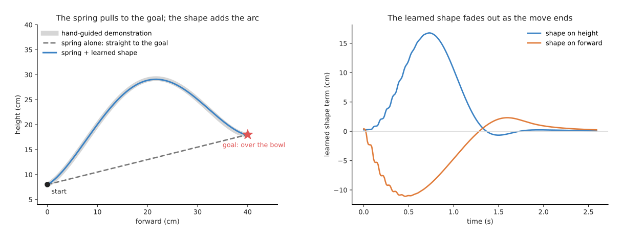
On the left, the blue DMP replay lies on the grey demonstration, and the largest gap between them is 5.1 millimetres (mm). On the right, the learned shape term is large in the first second, where the arc is, and it fades to nothing by the end.
Learning the shape from one demonstration#
The 30 heights are the only learned numbers, and a DMP needs only one demonstration to find them. Training works like this.
- Record the motion, and work out its speed and acceleration at each reading, from the differences between readings.
- Then at each reading, work out how much extra push the spring would need to produce exactly that acceleration, because this is the shape the model must learn.
- Then for each of the 30 bells, fit one number, which is a weighted average of that needed push, counting most the readings where that bell is strongest. This is locally weighted regression, with one small fit per bell, and it takes a fraction of a second.
So the result is 30 numbers per axis, 60 in all, plus the start, the goal and the duration.
A new goal, and a new speed#
Now move the bowl, give the DMP the new goal, and run it again, because nothing has to be retrained.
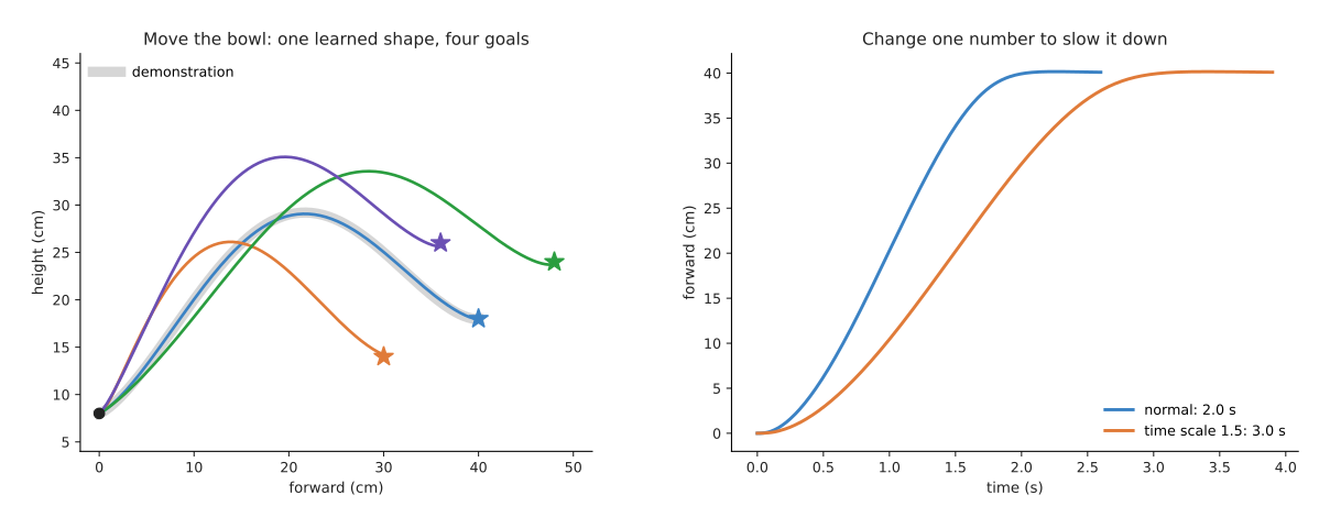
On the left, the same 60 numbers produce four paths, and each one lifts, arcs over and comes down to its own goal. The table below lists each goal, how close the DMP ends to it, and the highest point of the path, and you should read each row as one run.
| Goal (forward, height) | Distance from goal at the end | Highest point |
|---|---|---|
| 40 cm, 18 cm (the demonstration's goal) | 1.05 mm | 29.1 cm |
| 30 cm, 14 cm | 2.26 mm | 26.1 cm |
| 48 cm, 24 cm | 0.27 mm | 33.6 cm |
| 36 cm, 26 cm | 1.50 mm | 35.1 cm |
Every run ends within 2.3 mm of its goal, and the small leftover comes from the shape term, which is small but not exactly zero when the run stops.
On the right is time scaling, because a DMP has one number for its duration. Change it from 2.0 to 3.0 seconds, and the same motion runs one and a half times slower, while the path stays the same to within 2.1 mm. On an arm this is useful for a first slow try, or for slowing down near a person.
3. Probabilistic movement primitives: a path with a spread#
A probabilistic movement primitive (ProMP) was introduced by Alexandros Paraschos, Christian Daniel, Jan Peters and Gerhard Neumann in 2013. Unlike a DMP, it learns from several demonstrations rather than one, and it keeps not only the typical path but also how much the demonstrations varied at each moment. The word probabilistic means that it describes the chance of each possible path, and not only one path.
For example, a person hand-guides a cloth across a table in one wiping stroke, 8 times over. Each stroke swings sideways and comes back, but no two are the same. The script records the sideways position of the cloth at 100 moments in each stroke, with time written from 0 at the start to 1 at the end.
From demonstrations to a mean and a spread#
- Describe each demonstration with a few numbers, by placing 10 bells along the time axis. Then find the 10 heights that, when the bells are blended, best match the demonstration. This is an ordinary least-squares fit, and the largest mismatch over all 8 strokes is 5.8 mm.
- Now each demonstration is 10 numbers, so take the average of the 8 sets, and that average is the mean path.
- Then work out how the 10 numbers vary together across the 8 sets. This is their covariance, which is a table that says how much each number varies and which numbers tend to go up and down together, so it holds the spread.
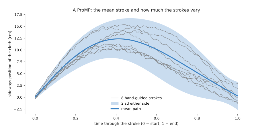
The band shows two standard deviations (sd) either side of the mean, so about 95 in 100 paths fall inside it. At the start the spread is 2.0 mm, because every stroke starts in the same place. Half-way through, the mean is 11.9 centimetres (cm) out, with a spread of 23.9 mm, and at the end the spread is 14.5 mm.
The spread tells the robot two things. Where the band is narrow the demonstrations agreed, so that part of the path probably matters, while where the band is wide the person did not care much, so the robot can bend the path there. Some controllers use this to hold the arm stiffly where the band is narrow and softly where it is wide.
Asking for a via-point#
The spread says where the path may bend, and a via-point says where it must not. A via-point is a point that the path must pass through at a set moment. Suppose a cup stands on the table, and the cloth must reach 15.5 cm out half-way through the stroke in order to wipe around it.
A ProMP answers this with conditioning: of all the paths the demonstrations allow, keep only those that pass through the via-point, and describe what is left. This is a short sum with the mean and covariance, with no retraining at all. It uses the same kind of update as the Kalman filter in Book 5, treating the via-point as one very precise measurement.
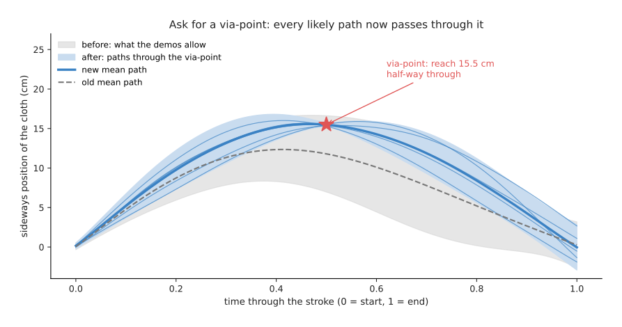
Before conditioning the mean at half-way is 11.9 cm, and afterwards it is 15.52 cm, with a spread of only 1.47 mm there. The thin blue lines are six paths drawn at random from the conditioned model, and all of them pass through the point. The new path does not simply jump to the point and back, because it bends smoothly, in the way the demonstrations varied, since the covariance says how each part of the path moves when another part does. The start and end spreads stay almost as they were, 1.8 mm and 14.4 mm.
A DMP can also reach a new goal, but it has no natural way to add a via-point in the middle. A ProMP instead can take any number of via-points, and a new start or goal is just a via-point at time 0 or 1.
4. How they are trained#
Sections 2 and 3 each learned from recordings, so this section says what those recordings must be like. A DMP needs one demonstration of the motion, and several can be averaged, although one is normal. It must start and end at rest, and it should be smooth, because the training uses the acceleration, and a shaky recording has a shaky acceleration. So people usually smooth the recording first, and training then takes well under a second.
A ProMP needs several demonstrations, usually 5 to 20, of the same motion with some natural variation. With too few of them the covariance is poor, because with 8 demonstrations and 10 numbers each, the spread is only a rough guess. The demonstrations must be lined up in time, usually by scaling each to run from 0 to 1. If people paused at different moments, a method called dynamic time warping can stretch the recordings so matching parts line up first.
Both learn each axis, or each joint, separately in their simplest form. But a ProMP can also learn how the joints vary together, by putting all the joints' numbers into one covariance.
Both kinds are usually learned in the hand's position, so that a new goal from a camera can be given in metres. They can also be learned in joint angles, when the arm's pose during the motion matters.
5. Where they are used on a robot arm#
- Pouring. A person hand-guides a pour once, then a camera finds the cup and the DMP is run with the cup's position as its goal, so the arc over the rim comes along for free.
- Wiping and polishing. A ProMP learns a stroke from several demonstrations, and a via-point then moves the stroke around an object on the table. The spread also tells a compliant controller where it may give way.
- Reaching a moved target. A reach-and-place learned as a DMP adapts at once when the target moves, even during the motion, because the goal can be changed while the DMP runs.
- Joining motions into a task. A task is often written as a finite state machine that runs one primitive after another: reach, grasp, lift, pour, put back. Each primitive is taught separately.
- Improving by practice. Because a DMP is only a few dozen numbers, a robot can try small changes to those numbers and keep the ones that do better. This is a small, fast form of the reinforcement learning covered in the movement chapter. It was one of the early successes of robot learning, for example for ball-in-a-cup games.
- Two arms together. A ProMP over both arms' positions learns how they move together, so that when one arm is told where to go, the other adjusts.
6. Primitives or a learned policy#
Section 5 listed the jobs primitives do, and the obvious competitor for all of them is a neural network. The movement chapter of this book describes behaviour cloning, which is a neural network that watches the camera and chooses the next move, trained on many demonstrations. Movement primitives and behaviour cloning both learn from demonstrations, but they suit very different jobs.
So the table below compares them, and you should read each row as one question, with the answer for each of the two.
| Question | Movement primitives | Behaviour cloning policy |
|---|---|---|
| How many demonstrations? | 1 for a DMP; 5 to 20 for a ProMP | usually 50 to several hundred |
| Does it need a camera? | no; the goal can come from anywhere | yes, usually, as the main input |
| What does it react to during the motion? | only its goal, via-points and timing | anything the camera sees |
| How many motions per model? | one smooth motion | a whole task, with many steps |
| Training time | under a second on a laptop | hours on a graphics card |
| Can you check it before it runs? | yes; you can compute the whole path first | no; it decides each move as it goes |
| Does it reach the goal? | a DMP always does | only if the training taught it well |
Primitives win when you have few demonstrations, the motion is a single smooth movement, and the only thing that changes is where it starts or ends. For example, pouring into a cup at a known place, wiping a stroke, or placing a part all fit that description. They also win when you must check the path before running it, or when you have no graphics card.
But a policy wins when the robot must react to what it sees during the motion, such as a towel that folds differently each time, a drawer that sticks, or an object that slides. It also wins for long tasks with many steps and choices, where writing a state machine of primitives would be long and fragile. And it wins when the task has more than one good way to do it, and the camera must decide which.
So the two are often combined, where a seeing model or a policy chooses the goal and a primitive then produces the smooth motion to reach it.
7. What goes wrong#
Section 6 said where primitives win, and this section says how they fail. A DMP generalises well only near its demonstration, so for a goal far away, or in a very different direction, the shape can look odd. The arc is added exactly as it was learned, and it is not rotated or stretched to suit the new direction, which is why the 36 cm, 26 cm goal above already arcs up to 35.1 cm. Some versions scale the shape by the distance to the goal, which fixes some cases and causes others, because when the start and goal are at almost the same height, the scaled arc shrinks to nothing. So the usual fix is to record demonstrations for the range of goals you need, or to learn in a frame attached to the target.
A DMP also does not know about obstacles, because the shape clears the bowl's rim only since the demonstration did. Extra repelling terms can be added near known obstacles, but for real collision checking a planner is needed.
A shaky demonstration gives a shaky replay, because the shape is learned from the acceleration, and differences of noisy readings are very noisy. So smooth the recording first.
A ProMP's spread is only as good as its demonstrations, because with few of them the covariance is a rough guess and conditioning can give strange paths. In particular, a via-point far outside the band forces the model to use shapes that it never saw.
Neither kind checks the joints' limits, because a DMP run with a short duration or a far goal can ask for more speed than the joints allow. Book 6's trajectory generation limits and a safety check are still needed underneath.
Orientation needs care, because the hand's turn cannot be learned as three separate angles without odd results near some poses. So DMP versions exist for turns written as quaternions, and most libraries include one.
8. Libraries#
You would use a library rather than write a DMP yourself, so the table below lists the real ones. Read each row as one library and what it provides.
| Library | Language | What it provides | Note |
|---|---|---|---|
| movement_primitives | Python | DMPs, including a version for the hand's position and turn, and ProMPs, in movement_primitives.dmp and movement_primitives.promp | from DFKI, by Alexander Fabisch; the most complete Python package |
| pydmps | Python | discrete and rhythmic DMPs, for example pydmps.dmp_discrete.DMPs_discrete | small and easy to read; good for learning |
| dmpbbo | C++ and Python | DMPs, plus black-box optimisation to improve them by practice | by Freek Stulp; aimed at practice on real robots |
But the methods are also short enough to write yourself, as the diagram script shows, because each of them is a few dozen lines of NumPy.
9. Why movement primitives, and what they cost#
The libraries make both kinds cheap to try, so this section says when to choose them. A movement primitive is a small model of one smooth motion, learned from one or a few demonstrations, where a DMP is a spring to the goal plus a learned shape and a ProMP is a mean path with a spread.
What they do for you: you teach a motion by hand-guiding it once or a few times. The motion reaches a new goal without retraining, can run faster or slower, and, for a ProMP, can pass through a new via-point. Training takes less than a second, and the whole path can be computed and checked before the arm moves.
The obvious alternative is a behaviour cloning policy, covered in section 6, which needs many more demonstrations and a camera but reacts to what it sees. The other obvious alternative is to write the path by hand as waypoints, covered in the next section. That needs no demonstration at all, but someone must be able to say where the path goes.
What they cost: each primitive is one motion, so a task needs several primitives and written code to join them. They react only to the goal, via-points and timing, and not to anything the camera sees during the motion. They also do not avoid obstacles or check joint limits. And they generalise only to goals near the demonstrated ones.
10. The written alternative#
Book 6's trajectory generation does the same job with no learning at all. Someone writes down a few waypoints, such as "lift to 25 cm, move over the bowl, lower to 18 cm", and the generator joins them with a smooth curve that obeys the joints' limits. For a new goal, the program simply moves the last waypoints. The written way wins when the path is easy to describe, such as a lift, a straight move and a lower, because it obeys the limits by design and can be read by anyone. The primitive wins when the motion is easier to show than to describe, such as the exact curve of a pour or the swing of a wiping stroke, and when a ProMP's spread is useful.
When the path must also avoid obstacles, Book 6's trajectory optimisation finds a smooth path that keeps clear of them. So some methods start that optimisation from a primitive's path, and the result then stays close to the demonstration.
11. Where to read next#
- Behaviour cloning learns a policy that reacts to the camera, from many demonstrations.
- The movement models overview compares every kind of learned policy.
- Mixture models and hidden Markov models learns a motion with Gaussian mixture regression, and splits a demonstration into steps.
- Where the data comes from explains teleoperation, the other common way to record demonstrations.
- Book 6's impedance and force control explains the springs and dampers used in the controller that follows a primitive, and in hand-guiding itself.
12. Using it in Python#
Section 2 built a dynamic movement primitive out of a spring and a learned shape, section 3 turned several demonstrations into a mean path with a spread, and section 8 named the libraries. This section shows the calls in the most complete of them, so that after reading it you can learn a primitive from a recording and play it back to a new goal.
The package is movement_primitives, the DFKI one from section 8. It is
installed with pip install movement-primitives, and it also needs
pytransform3d, because its DMP module imports that for the version that handles
the hand's turn as well as its position.
import numpy as np
from movement_primitives.dmp import DMP
from movement_primitives.promp import ProMP

# T holds the time of each recorded sample, Y the recorded position,
# one row per sample and one column per dimension.
dmp = DMP(n_dims=2, execution_time=1.0, dt=0.01, n_weights_per_dim=10)
dmp.imitate(T, Y)                   # section 2's learned shape
dmp.configure(start_y=Y[0], goal_y=np.array([0.0, 1.5]))   # section 2's new goal
T_out, Y_out = dmp.open_loop()      # play it back

# Ts and Ys are lists with one entry per demonstration.
promp = ProMP(n_dims=2, n_weights_per_dim=10)
promp.imitate(Ts, Ys)
mean = promp.mean_trajectory(T)     # section 3's mean path
spread = promp.var_trajectory(T)    # and the variance around it
conditioned = promp.condition_position(np.array([0.5, 0.5]), t=0.5, t_max=1.0)
The configure call is what section 2 called the useful property of a DMP,
because you learn the shape once from one demonstration and then ask for a
different goal without recording anything new. The condition_position call is
section 3's via-point, and it returns a new ProMP whose paths all pass through
the point you named, which is why the result is assigned to a new variable rather
than changing promp in place.
The library gives you the parts that are tedious to get right: the phase
variable, the basis functions spread along it, the regression that turns a
recording into weights, and the numerical integration that plays the result back.
It also gives you the probabilistic algebra behind condition_position, which is
the longest piece of arithmetic on this page.
What you have to collect is the demonstration, and for a ProMP several
demonstrations of the same motion. They must be resampled onto a common time
vector, because imitate pairs each row of Y with the matching entry of T,
and a ProMP needs the demonstrations to line up in time. Section 4 described that
preparation, and section 7 added that you should smooth the recording first,
because the shape is learned from the acceleration and a shaky recording gives a
shaky replay.
What you have to decide is n_weights_per_dim and execution_time. More weights
follow the demonstration more closely, so they also copy more of whatever shake
is left in it, while too few smooth away the part of the motion that mattered.
execution_time sets how long the playback takes, and section 2 showed that
changing it slows or speeds the whole motion without changing its shape. If you
would rather see the arithmetic than use it, section 8 noted that each method is
a few dozen lines of NumPy.